September 3, 2008
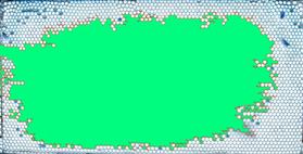
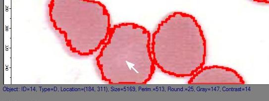
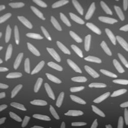
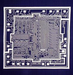
A few days ago I was contacted by a representative of a biotech company. He was interested in figuring out how Pixcavator can help them to automatically carry out a function that they currently do manually. They were looking for a method to automatically measure, document, and summarize characteristics of a certain kind of fibers in digital photos. Specifically, they needed: length and width, along with some very basic statistical data (size, length, width, ratio length to width, etc.), and graphical representations of the data (histograms). The image is below.
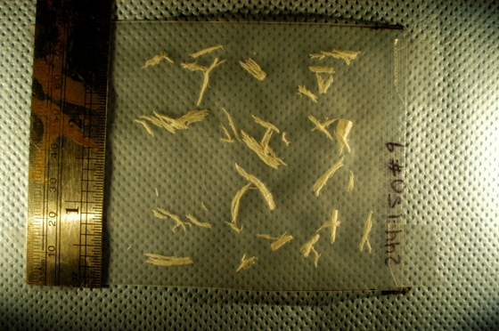
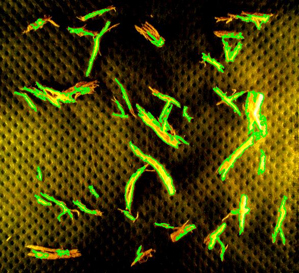
Capturing fibers wasn’t hard. Some of the irrelevant features are also captured but they were easy to filter out. The results would be better with better images: uniform dark background, less reflection etc. Separating fibers from each other would be a challenge; fortunately, the fibers were to be measured as “clumps” if they are attached to each other.
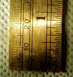 Averages are computed automatically but to have the answer in inches I had to calibrate the image. For that I used the ruler in the image (all the computations in the spreadsheet). I just found the end points of the one inch part of the ruler: from (193,235) to (196,44). This gives the distance Averages are computed automatically but to have the answer in inches I had to calibrate the image. For that I used the ruler in the image (all the computations in the spreadsheet). I just found the end points of the one inch part of the ruler: from (193,235) to (196,44). This gives the distance
SQRT( (196-193) * (196-193) + (235-44) * (235-44) ) = 191 pixels.
So,
1 inch = 191 pixels.
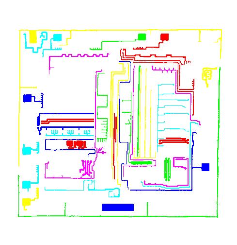
Then I recomputed the averages. The result:
Average width: 0.02, average length: 0.52 inches.
This does not seem too far off. There may be a discrepancy in the way people understand width and length though. Basically, we consider the area and the perimeter of the object, then find the rectangle with these measurements, then take its width and length. Sometimes this is called the ribbon length.
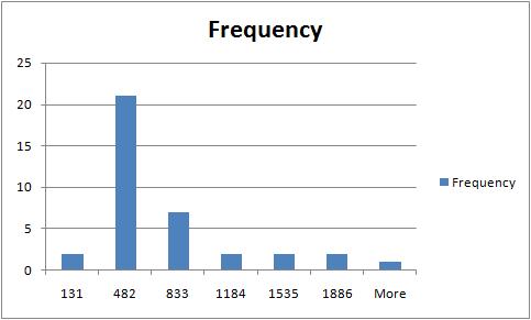
The rest of the required output is easily acquired after some Excel work. The histogram of sizes (in pixels) of fibers is below.
For other examples, see our wiki.
August 24, 2008
Previously we discussed the watershed algorithm for binary images. One thing that wasn’t explained was where the name comes from.
We start with the following approach. According to Gonzales and Woods: “we think of a gray scale image as a topological surface, where the values of f(x,y) are interpreted as heights.” This is good (except the redundant “topological”) and quite clear. Mathematically, if f(x,y) gives the value of gray of the pixel (x,y), we simply end up with the -graph of f (remember precalc?).
Next, we find the “catchment” basins. Mathematically, these are minimum points of the surface. However, to find basins’ borders we need to find the ridge lines that separate them. Mathematically, those are lines that go from one maximum point to another via the saddle points.
To summarize, we create a surface from the image by using the value of gray at a given pixel as the height of the surface above it. The light areas are the peaks and the dark areas are the valleys. Next, we flood the valleys, gradually. As we do that, we don’t allow the water to flow from one valley to another. How? By building dams. These dams will break the image into regions each containing a single valley. That’s image segmentation.
Let’s now take a look at the Wikipedia article: “The watershed algorithm is an image processing segmentation algorithm that splits an image into areas, based on the topology of the image.” First, any segmentation algorithm splits an image into areas. Second, any segmentation should be based on the topology of the image. So, what’s left is “The watershed is an image segmentation algorithm”.
The next sentence is “The length of the gradients is interpreted as elevation information.” Wait a minute, that’s not the same! The length of the gradient is the steepness of the surface. In the next sentence however the article seems comes back to the standard approach: “During the successive flooding of the grey value relief, watersheds with adjacent catchment basins are constructed.” And then again: “This flooding process is performed on the gradient image…” Using the gradient as the surface is an alternative approach to the watershed, so this must be a mix-up. Another approach is using the distance function for binary images.
We’ll discuss these issues in the next post.
August 20, 2008
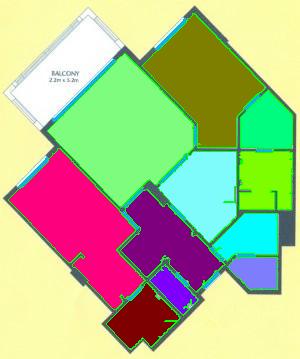
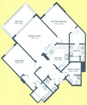 As a suggestion from one of our users, we used Pixcavator to analyze floorplans. The task is very simple – measure the rooms. As a suggestion from one of our users, we used Pixcavator to analyze floorplans. The task is very simple – measure the rooms.
Measuring irregular (or even regular) isn’t easy for a person because unless all rooms are rectangular one needs know some geometry. If the corners aren’t 90 degrees, you may have to measure them and then (OMG!) use trigonometry. The walls can also be curved. If the curves are known, all you need is calculus (OMG!!). It is unlikely that the formulas for the curves come with the floorplan, so digital image analysis seems inevitable.
The results are below. Of course, I had to “close” the doors first.
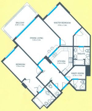 
Calbration wasn’t addressed though.
August 17, 2008
The paper is A review of imaging techniques for systems biology (BMC Systems Biology 2008, 2:74) . Pixcavator is listed in “Table 2 - Overview of microscopy image analysis software” along with a few other companies/products. All the usual suspects are here: Image-Pro from Media Cybernetics, ImageJ, CellProfiler, Clemex Vision. The rest are less familiar and some of the companies are mostly about hardware. The paper itself is about imaging methods not image analysis. Even though this is not a endorsement by any stretch of imagination, it’s nice to be mentioned. (Smart people will also notice a few products that aren’t mentioned.) BMC stands for BioMed Central.
August 14, 2008
The updated interface is the first thing that you notice. All buttons and sliders are arranged in groups accompanied by headers. Text and tooltips were improved throughout.
The RGB channel analysis was completed to include all three channels. Just click a button in the Analysis tab for the color you want.
A new, “Max growth rate”, slider was introduced. Let me explain what it is. As you may remember object in the image are allowed to grow – from one level of gray to the next - up to the extent set by the slider. For example, the object will grow until it’s both larger than say 100 pixels and has contrast above 20. Now, this is a totally different kind of slider. If you choose 10, the object will be allowed to expand – from one level of gray to the next - as long as its size grows by 10% or less. Roughly, the expansion stops once the contour reaches a sharp edge. There will have to be more written about this after some testing. (To reproduce results you obtained with the older versions of Pixcavator just keep this value at 0.)
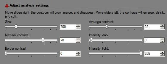
A new header is Data filtering. There are only two buttons here currently – Unmark dark and Unmark light. For convenience they were redesigned as follows. These are toggle buttons so that you can choose to concentrate on only, say, light objects without having to unmark dark every time you change the settings. There is more to come here.
The analysis summary now includes the mean values and standard deviations of all the main characteristics of objects (marked only).
The way contours are plotted was improved. Now red and green contours never overlap no matter how close they are to each other.
A noticeable speed-up was achieved, in both image analysis and graph analysis part. The memory usage was significantly reduced. There were also numerous minor improvements.
August 10, 2008
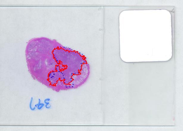
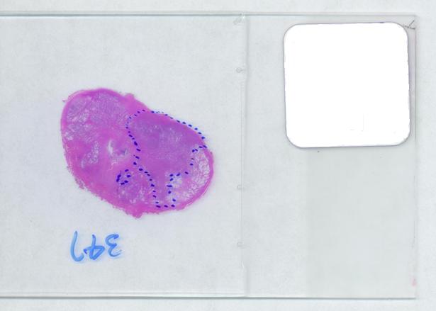 The first picture explains what normally happens when a prostate tumor has to be evaluated. The prostate is cut into thin slices and the slices are put on pieces of glass. Next, the doctor outlines the tumor within the prostate with a marker. Finally, the area of the outlined region is evaluated in each slice and the volume of the tumor is estimated. The first picture explains what normally happens when a prostate tumor has to be evaluated. The prostate is cut into thin slices and the slices are put on pieces of glass. Next, the doctor outlines the tumor within the prostate with a marker. Finally, the area of the outlined region is evaluated in each slice and the volume of the tumor is estimated.
Evaluating the area of the tumor with a naked eye will give you a very low accuracy. Best one can do to improve that is to superimpose a grid over the image and count the number of squares that fall into the tumor. Then the accuracy will be inversly proportional to the size of the square but the smaller the square the more complex the manual counting will be.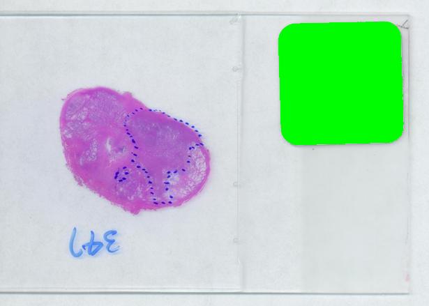
Digital image analysis is a necessity here.
I analyzed the shrunk version (615×439) of the image with Pixcavator followed by some back-of-the-envelope calculations.
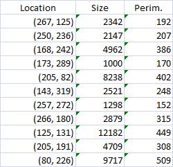
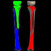
The critical part of analysis is the calibration. For that I used the square label in the image. It is known that its side is 2.2 cm. Now, I pushed the size slider almost all the way to the right and ended up with just one object -the label (green). Its area according to the table is 29,516 pixels. If we ignore the round corners (introducing some error here, unfortunately), it is a square. So 29,810 pixels = 2.2 * 2.2 = 4.84 sq cm.
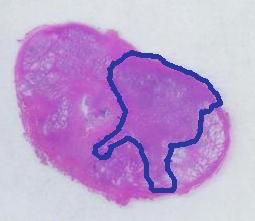
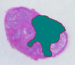
Next, the tumor. The dotted line is made solid using MS Paint. The you run Pixcavator. The contour has the area of 9,491 pixels. So, it is 9,491 * 4.84 / 29,810 = 1.54 sq cm.
 The end. The end.
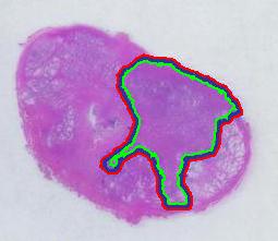
There is still the issue of error however. The error produced by hand drawing is estimated in the next experiment. Pixcavator evaluated the area on the outside of the curve (9,774) and on the inside (7,112). Hence the area of the curve is (9,774– 7,112) / 9,774 = 27% of the outside of the tumor. That’s the error.
It seems too high!
To verify the result, let’s approach from another direction. The perimeters are 542 and 530 respectively. Then the average thickness of the line is (9840-7342)/536 = 4.7 pixels. Examination of the image confirms this number. Of course, the error can be easily cut down by making the line 1/2 thinner but it will still remain high…
That brings us to the possibility of discovering the tumor within the prostate automatically. To be precise, the procedure would be semi-automatic not automatic, and it is the doctor who would make all the decisions. He chooses the contours and Pixcavator just counts pixels. What it gives you is a procedure that is somewhat simple – moving sliders until you have a good fit – and quite accurate – if the fit is good. Finding a good contour won’t require training but just a bit of practice. The last image shows that this approach isn’t totally unreasonable…
July 29, 2008
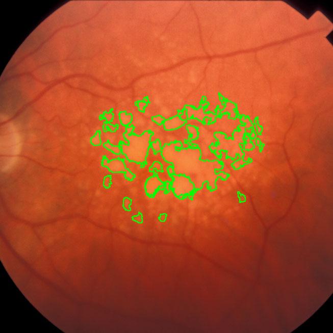
During a retina inspection one of the most common pathology is Drusen deposits. Some computer assisted methods have been created to solve this problem and especially avoid the subjectivity of the doctors (”MD3RI a Tool for Computer-Aided Drusens Contour Drawing”) [1].
An image from this paper is below:
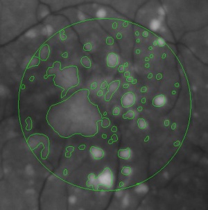
Pixcavator easily produces similar results:
Another example is ice cracking (thanks to Nikolay Makarenko for the idea). The image is analyzed with Pixcavator with settings 596-63.
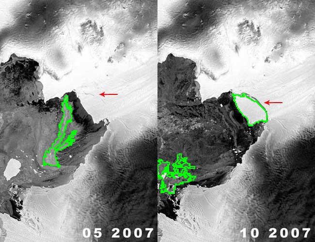
An iceberg is born!
These kind of examples will appear in the wiki under Case studies.
July 27, 2008
The paper (PDF, 10 pages, 360K) describes the algorithm behind Pixcavator. The algorithm is presented in detail in the wiki but this is a new and improved exposition. I reconsidered some of the terminology, re-wrote the pseudocode, and improved illustrations. There is also a gap in the wiki - when an edge is added to the image, case 4 is missing. I’ll have to re-write a few articles. The presentation in the paper is less detailed (in terms of examples, images etc) but it is a bit more thorough.
Abstract: The paper provides a method of image segmentation of binary and gray scale images. For binary images, the method captures not only connected components but also the holes. For gray scale images, there are two kinds of “connected components” – dark regions surrounded by lighter areas or light regions surrounded by darker areas.
The long term goal is to design a computer vision system “from first principles”. The last sentence in the abstract is one such principle. Keep in mind (of course) that if every dark region surrounded by a lighter area is an object, it does not mean that every object is a dark region surrounded by a lighter area (or vice versa). In a way, these are “potential” objects and you still have to filter and/or group them to find the “real” ones. So there must be more first principles.
The paper does not go far beyond this stage. The main step is – all potential objects are recorded in the “topology graph” (“frame graph” in the wiki). Then only one method of filtering is presented (the one based on size).
All feedback is welcome.
July 20, 2008
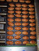
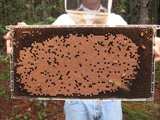 This came as a question from one of our users. The picture explains the problem: there is a bee frame with several hundred sealed brood. They are visible as tan hexagons (the dark circles are empty cells). Now, count them! Just like that – an outdoors photo taken with a regular digital camera, no registration, no calibration, etc. This came as a question from one of our users. The picture explains the problem: there is a bee frame with several hundred sealed brood. They are visible as tan hexagons (the dark circles are empty cells). Now, count them! Just like that – an outdoors photo taken with a regular digital camera, no registration, no calibration, etc.
The problem is interesting but also quite challenging. The sealed cells aren’t separated enough from each other to count them one by one with 100% accuracy. For that 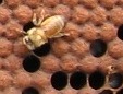 the image would need a higher resolution. If, however, the goal is just an estimate, Pixcavator can help. Then the task is less about counting and more about measuring… and some elementary school math. the image would need a higher resolution. If, however, the goal is just an estimate, Pixcavator can help. Then the task is less about counting and more about measuring… and some elementary school math.
First I cropped the image. Then I analyzed it with 100-130 settings, no shrinking. The result is 311 dark objects (clusters of empty cells) with the average size 1,255. So the total area of the empty cells is
311*1,255 = 390,305.
Since the image is 1,394×709, the area covered by sealed cells is
1,394*709 - 390,305 = 598,041.
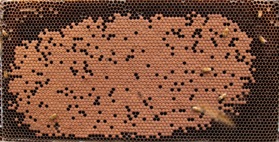 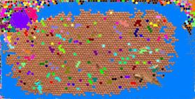
Just in case I decided to validate this number from another source. I analyzed the negative with 100-110 settings. Then I just picked the largest object in the table - the cluster of all sealed cells. Its area is 613,814. Since the empty cells inside of this area aren’t taken into account, the result is higher than the first estimate. The difference is however less than 3%.
At this point you need to estimate the size of a cell. Looking at a few individual cells in the table may give you an estimate, but it would take some work with Excel. Instead I did actual measuring - on the screen. I counted 10 cells in a row and measured the length with a ruler - 34 mm. So each cell is about 3.4×3.4 mm. Next I measured the image - 270×136 mm. So the number of cells is
270*136/(3.4*3.4) = 36,720.
(The user won’t need this computation because the actual number is known). Then the size of the cell is
(the size of the image in pixels) / (the number of cells) = 1,394*709/36,720 = 269.
Finally, the number of sealed cells is
(the total area) / (the size of each) = 598,041/269 = 2,223.
The hand counted number is 2,198. The error is about 1%!
You can reproduce these results with Pixcavator version 3.0 or earlier and this full size image: http://inperc.com/wiki/images/7/7d/Bee_brood-cropped.jpg.
July 13, 2008
On several occasions I was asked: Why wouldn’t we add a second slider to the size ruler? The logic is very convincing: “the first slider removes objects from analysis that are too small - with the second slider you can exclude objects that are too large”. There are real life problems that need this kind of analysis.
What is wrong with this idea? The problem is that the idea is “binary”. If the image is binary, excluding larger objects is a simple operation. We however deal with gray scale images. Sometimes objects in gray scale images look just like ones in binary images but often they have no well defined boundary. No well defined boundary – no well defined size!
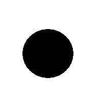 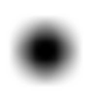  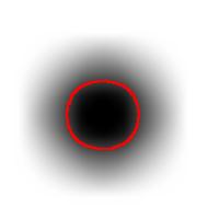 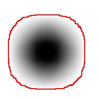
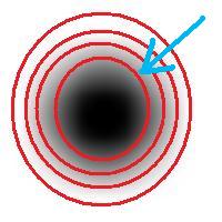
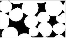
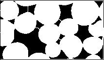
For example, this is a binary image of a circle and that is the same image blurred. There is clearly just one object here and it looks like circle. But what’s its size? It could be a small spot in the middle, or large circle, or it could be the whole image (why not?). If there are several objects like that, we can’t filter them based on larger/smaller comparison. As a result, we can’t even count them properly because without measuring we can’t tell noise from what’s important.
But wait a minute, of course, our software counts objects! So, how?
The user sets a lower bound on sizes of objects he considers important. Anything smaller is noise. What the user doesn’t know (but should) is what is an object. The definition of an object is in fact very simple:
An object is either a dark region surrounded by lighter area or a light region surrounded by a darker area.
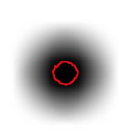
For example, in the above image we have many-many circular objects. Too many, in fact, because we know that there is only one! So, the objects that we’ve found aren’t actual objects but “potential” objects. At this point we need to select just one. How?
We use the bound chosen by the user! We exclude all potential objects that are smaller than this bound. Good, but even now we still have multiple objects. What do we do? We just take the smallest!
Roughly, once the bound is set, the object is allowed to grow until its size is over the bound.
Suppose the bound is 100. Then what we present as the output is objects larger than 100 BUT as close as possible to 100. If the gray level changes very gradually, the objects’ sizes end up almost exactly equal 100. If this is the case, having an upper bound (say 200) in addition to the lower bound would not change the outcome…
That’s why only a single slider for the size is present. If object A is larger than object B, A is at least as important as B. A priori, all things being equal.
The second slider is for contrast and it operates in the exact same way: the object is allowed to grow until its contrast is over the bound. The logic is the same as before: a priori, if object A has a higher contrast than object B, A is at least as important as B.
OK, but what about those real life situations when you need to exclude larger objects? That’s when you turn from image analysis to data analysis. Of course, you’d have to make sure that you have captured all objects that you care about. That’s the hard part.
The data analysis stage is the easy part. If you have captured some noise or objects that you want to exclude, that’s OK. Now you simply filter the objects on the list based on any characteristic you want. Excel has plenty of tools for that. For example, the size is too large or too small. Or the perimeter, the contrast, the roundness, the intensity. Maybe you want only the objects from 100 to 200 pixels in size. Or maybe you are only interested in the objects within 300 pixels from the center of the image. All is easy at this stage.
July 6, 2008
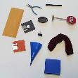
Pixcavator is a light-weight (336K here) image explorer. Below I list new features and other modifications.
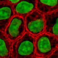
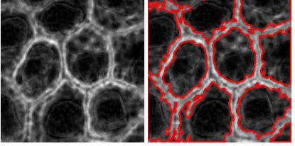
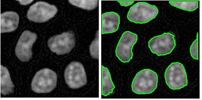
RGB channel-by-channel analysis. It’s an experimental feature, so that you can only use the red or the green for now. This is important for some applications such as microscopy. Different features are sometimes better revealed in different channels. Below: original, analysis in red channel, analysis in green channel.
Analysis summary to include some statistics. The output table contains only the raw data about each object. Of course, if you save the data to Excel, you can get anything from it: average of all columns, histograms, etc. We thought that it would be nice to be able to preview some data: average values of size and contrast. There will be more.
Data displayed based on the location of the mouse. That’s another very convenient feature. You used to have to mark/unmark object in the image and then find the row in the table to see the objects’s measurements. That’s not fun if the table is a hundred rows long. Now you let the mouse hover over the object of your interest and the data from the table is displayed right beneath the image.
Coloring objects. This feature was previewed a couple of weeks ago.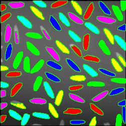
Hiding contours. To see the original image you used to have to go to the Analysis tab. Now you can flick it on and off to see what is hiding under the contours. The marking/unmarking of objects is unaffected.
Some sliders removed. The sliders for roundness and saliency haven’t been used a lot as far as I know. The complexity they add did not seem worthwhile. It does not mean that there will be always just the two sliders. The development of new characteristics for the sliders is under way. They will only be added if they make a significant improvement over what we have now. At least one new slider is coming in the next release.
Shrink slider modified. The shrink slider used to give you the shrink factor in terms of the area of the image. Now if you set itat 2, both of the dimensions will be cut in half while the area (and the processing time) will be cut by 4. This seems simpler. It is also preset to cut the processing time to 10 seconds or less. It seems like 99% of the time the resolution is excessive relative to the features being sought.
June 29, 2008
According the ImageJ site: “Watershed segmentation is a way of automatically separating or cutting apart particles that touch”.
Suppose black is the particles and white is the background. The the procedure is fairly simple.
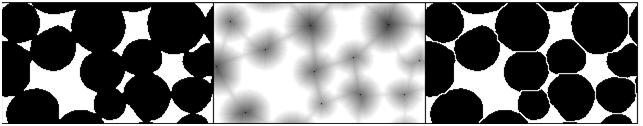
First, for each pixel compute the distance to the nearest white pixel. This is called the distance function. It’s a scalar function of two variables.
Next, find the maximum points of this function. Each of these pixels will become the center of a particle.
You carry out multiple rounds of dilation that gradually grow these particles. The dilation has two restrictions. First, the particles aren’t allowed to grow beyond the original set of black pixels. This way we guarantee that we end up with the same set of pixels except it has been “cut” into pieces. Second, a new pixel isn’t added if it’s adjacent to a pixel that belongs to another particle. This way the particles start to “push” onto each other but never overlap.
The tricky part of the last restriction is that the growth rate will have to be different for particles of different sizes. Otherwise, two particles will always be separated by a cut exactly half way between their centers. That wouldn’t make sense if one is significantly larger than the other. Roughly, the dilation rate should be proportional to the value of the distance function.
Some questions remain. For example, how does one efficiently find the maxima? Everything is discrete, so forget about partial derivatives etc. You have to visit every point.
How does one deal with particles that are simply noise? If you remove all small particles, you may have nothing left. One answer is to discard the maxima with low values of the distance function.
Another issue is typical for many image analysis techniques. Once again to quote the ImageJ site, “Watershed segmentation works best for smooth convex objects that don’t overlap too much.” Basically, you have to view (analyze!) the image yourself and decide ahead of time whether the method is appropriate. There is a good reason to be cautious – non-convex particles may cause the watershed method to produce undesirable results.
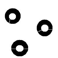
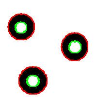
You have to choose ahead of time whether you have white or black particles. If you don’t do it correctly, you end up with non-convex black “particles”. The result of watershed segmentation isn’t what you expect:
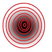
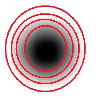
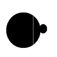
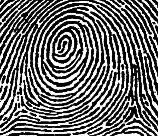
It is also easy to think of an image (rings) that can’t possibly be analyzed correctly by watershed regardless of the black/white choice:
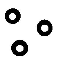  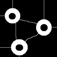
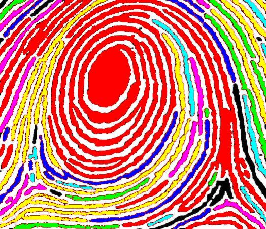
Needless to say that the topological method produces the correct segmentation here:
 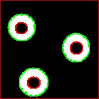
It can’t however separate particles yet (the stuff will appear in the wiki under Robustness of topology).
June 22, 2008
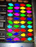
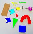
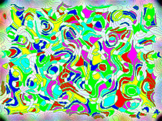
The next version of Pixcavator is to be relased in a few weeks. A new feature that I want to preview is Coloring Objects. Once objects are found, you can do anything with them. So, it was easy to implement (the objects are colored randomly). And it’s definitely an amusing feature. It can also be helpful.
This tool can help you confirm that your image segmentation is correct:
A more intricate segmentation:
Coloring combined with background removal:
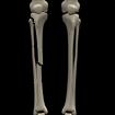
Something more amusing: recoloring objects and discovering a broken bone:
Just for fun:
For more examples, see our Image Gallery.
June 8, 2008
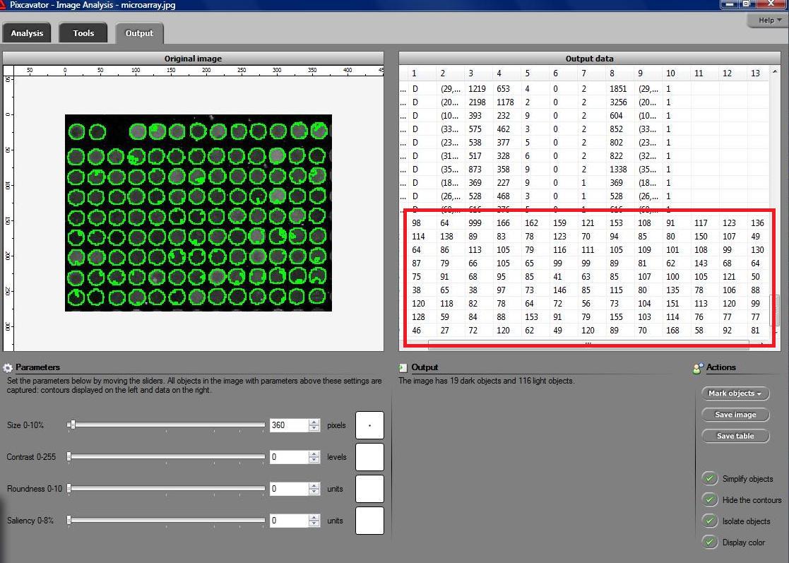
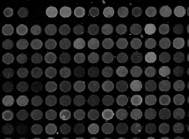 Microarrays (microplates etc) are plastic rectangles with a grid of “wells” containing biological materials. When another biological or chemical substance is added to these cells, the reaction is captured in digital images. For example, various concentrations of a chemical or a drug are added to the wells containing biological cells. The cells then start to divide faster, or slower, or simply die. The result affects the color of the substance in each cell. The image analysis automatically captures this data and draws conclusions. For example, you can pinpoint exactly at what concentration the drug becomes toxic. It’s like hundreds experiments in one! Appropriately, this is also called high throughput screening. Microarrays (microplates etc) are plastic rectangles with a grid of “wells” containing biological materials. When another biological or chemical substance is added to these cells, the reaction is captured in digital images. For example, various concentrations of a chemical or a drug are added to the wells containing biological cells. The cells then start to divide faster, or slower, or simply die. The result affects the color of the substance in each cell. The image analysis automatically captures this data and draws conclusions. For example, you can pinpoint exactly at what concentration the drug becomes toxic. It’s like hundreds experiments in one! Appropriately, this is also called high throughput screening.
I’ve been working on a related project for one of our clients and I would like to present a modified version of Pixcavator. First it captures all the wells in the form of a list with all the data about them – in the usual way. Then it displays the gray level (intensity) for each well – according to its position in the microarray. Of course, instead of intensity you can display other characteristics of these objects: the average intensity, or the standard deviation, or the average color (for color images), etc.
The point of the post is this: the hard part of collecting the data about the objects is taken care of by Pixcavator - the rest is a easy exercise with the Pixcavator SDK.
May 23, 2008
We are happy to announce the release of cellAnalyst version 2.0!
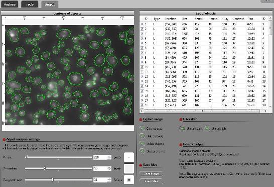
Just to remind you, cellAnalyst by AssaySoft Inc. is an advanced image-mining tool in a user-friendly package. It is designed to automate the analysis of digital images, especially ones coming from cell biology. It works as follows:
- The images are initially presented in a photo album format.
- With just a few clicks, cells have been detected, captured, and measured.
- The cells are listed in a table along with their characteristics.
- Each such table is saved as an entry in a searchable database.
Items 2 and 3 came originally from Pixcavator.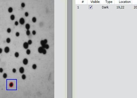
Now, the main new feature in version 2.0 is Partial Analysis. Analysis of images may be a time consuming task especially when the analysis setting have to be determined by trial and error. To reduce the processing time, one may start with analysis of just a portion of the image. The user draws a rectangle around a cell, and the analysis instantly determines its size and contrast. These two numbers are then used as the settings for the analysis of the entire image. More will appear in the wiki under Analysis strategy.
Other improvements are these:
- The roundness of every object found in the image is computed and displayed in the output table.
- Image enhancement functions are added: you can adjust brightness, contrast, color balance, gamma correction, and saturation.
- The estimated processing time is computed and displayed so that the user can plan ahead.
- Annotation can be added to images; it can later be used for search.
Download cellAnalyst here.
Feedback will be appreciated!
— Next Page » |
|
|


")


