September 10, 2008
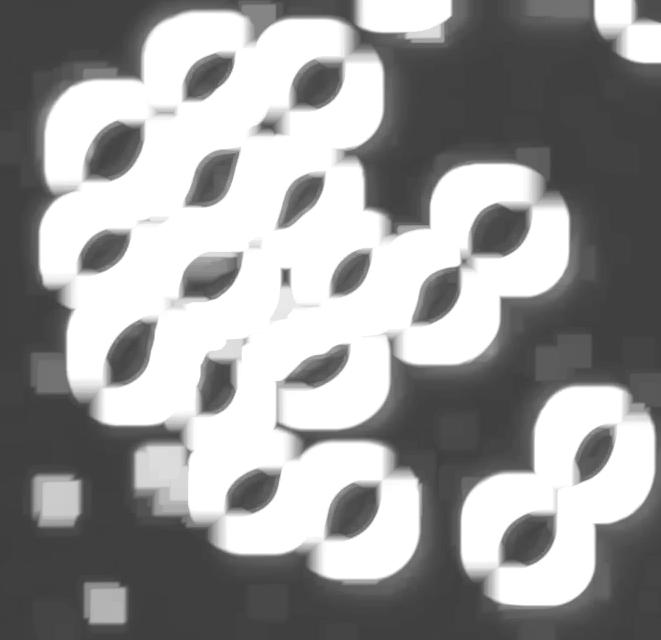
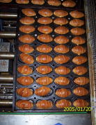
These are fixed red blood cells. The task is to count them with Pixcavator. They average 7.7 microns in size and were photographed unstained with differential interference contrast lighting. I had to crop the image to ensure reasonable processing times.
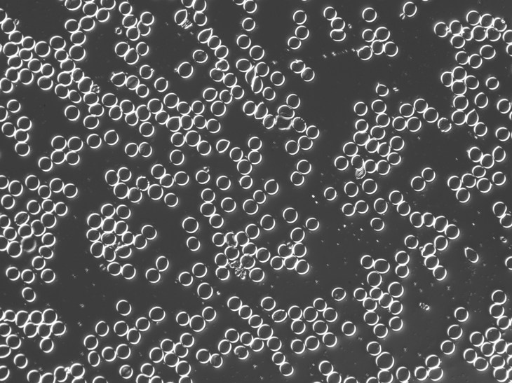 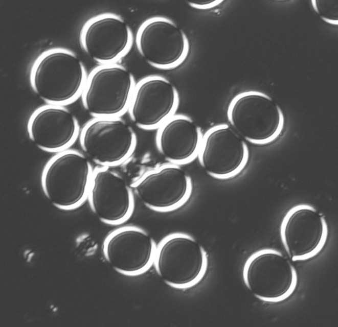
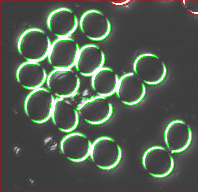
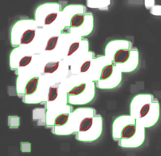
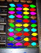
The quality of the image is good, but there is still a problem with the image. Each cell is captured by two light semicircles. These two semicircles aren’t connected to each other however (because the light comes from one direction?), so there are no full circles. The result is that cells can’t be treated as objects and they aren’t captured by the software. In the left image, there should be red contours for each of the cells like in the image on the right.
One way to get around this is to count the semicircles themselves (2 per cell). I ran Pixcavator with the following settings: 1000 for area and 100 for contrast.
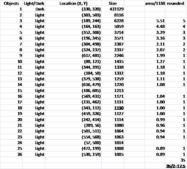
The problem with counting semicircles is that many of some of them touch each other so that they form clusters. These clusters are what’s captured by Pixcavator. To deal with this problem I needed some extra computation that followed the analysis. In the last column of the saved spreadsheet (table below) I divided the areas of the clusters of semicircles by the area of one semicircle (“1030”). The total number of semicircles found this way was 35. Then the estimate was 17.5 versus 17 of manual count.
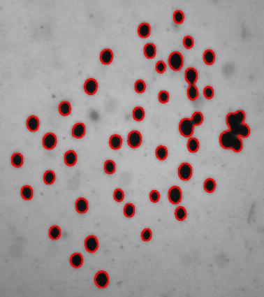
Another way to handle the problem is to start with some preprocessing. Erosion makes the light semicircles grow, they merge and form circular regions. Inside of those lie dark objects captured by Pixcavator. They correspond to cells.
I did 15 rounds of erosion (I had to use Pixcavator’s feature because ImageJ does erosions for binary images only). 15 is a lot as you can see.
Then I analyzed the image with the following settings: contrast 27, saliency 6768. The erosions, however, created several artifacts that had to be unmarked.
This method is more straightforward. With it, however, it is harder to get good results without manual intervention.
Live cells in the next post.
For other examples, see our wiki.
August 20, 2008
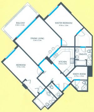
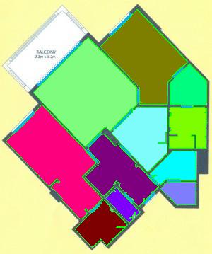
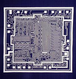
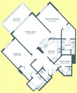 As a suggestion from one of our users, we used Pixcavator to analyze floorplans. The task is very simple – measure the rooms. As a suggestion from one of our users, we used Pixcavator to analyze floorplans. The task is very simple – measure the rooms.
Measuring irregular (or even regular) isn’t easy for a person because unless all rooms are rectangular one needs know some geometry. If the corners aren’t 90 degrees, you may have to measure them and then (OMG!) use trigonometry. The walls can also be curved. If the curves are known, all you need is calculus (OMG!!). It is unlikely that the formulas for the curves come with the floorplan, so digital image analysis seems inevitable.
The results are below. Of course, I had to “close” the doors first.
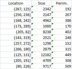
Calbration wasn’t addressed though.
August 3, 2008
Image analysis and computer vision is the extraction of meaningful information from digital images. One of the most prominent application of computer vision is in medical image processing - extraction of information for the purpose of making a medical diagnosis. It can be detection and measurement of tumors, arteriosclerosis or other malign changes or it can be identifying and counting cells, etc. Other main areas are industrial machine vision (automatic quality inspection, robotics, etc) and the military (missile guidance, battlefield awareness, etc).
The science of computer vision consists of an abundance of image analysis methods. These methods have been developed over the years for solving various but often narrow image analysis tasks. The result is that these methods are very task specific and seldom can be applied to a broad range of applications.
Our conclusion is then that as a discipline computer vision lacks a solid mathematical foundation.
Our long term goal is to design a comprehensive computer vision system “from first principles”. These principles come initially from one of the most fundamental fields of mathematics, topology. The idea is that just as mathematics rests on topology (and algebra), computer vision should be built on a firm topological foundation.
Algebraic topology is a well established discipline within mathematics. Its main computational tools have been implemented as software (CHomP, Computational Homology Project, and others). However, this theory and these tools are only applicable to binary images.
A framework for analysis of gray scale images has been under development. It is called Pixcavator. It includes both an image analysis software and an SDK. Pixcavator was into a product that also includes image management and database capabilities.
Some further issues remain. Future projects include the development of:
- protocols for applying the framework for specific tasks (e.g., tumor measurement),
- new methods that resolve the ambiguity of the boundaries of objects in gray scale images,
- integration of the existing image analysis methods into the framework,
- a framework for video (first binary, then gray scale, etc),
- a framework for color images (and other multichannel images),
- a framework for 3D images (first binary, then gray scale, etc).
July 29, 2008
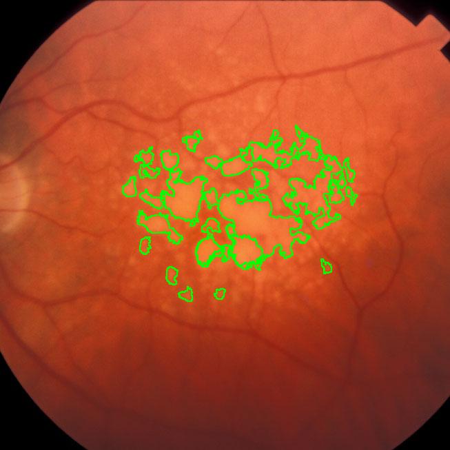
During a retina inspection one of the most common pathology is Drusen deposits. Some computer assisted methods have been created to solve this problem and especially avoid the subjectivity of the doctors (”MD3RI a Tool for Computer-Aided Drusens Contour Drawing”) [1].
An image from this paper is below:
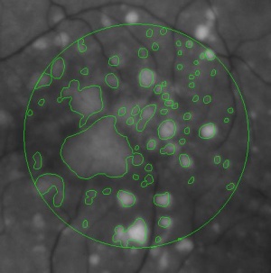
Pixcavator easily produces similar results:
Another example is ice cracking (thanks to Nikolay Makarenko for the idea). The image is analyzed with Pixcavator with settings 596-63.
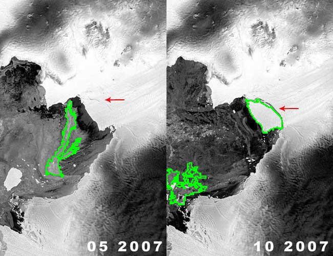
An iceberg is born!
These kind of examples will appear in the wiki under Case studies.
July 27, 2008
The paper (PDF, 10 pages, 360K) describes the algorithm behind Pixcavator. The algorithm is presented in detail in the wiki but this is a new and improved exposition. I reconsidered some of the terminology, re-wrote the pseudocode, and improved illustrations. There is also a gap in the wiki - when an edge is added to the image, case 4 is missing. I’ll have to re-write a few articles. The presentation in the paper is less detailed (in terms of examples, images etc) but it is a bit more thorough.
Abstract: The paper provides a method of image segmentation of binary and gray scale images. For binary images, the method captures not only connected components but also the holes. For gray scale images, there are two kinds of “connected components” – dark regions surrounded by lighter areas or light regions surrounded by darker areas.
The long term goal is to design a computer vision system “from first principles”. The last sentence in the abstract is one such principle. Keep in mind (of course) that if every dark region surrounded by a lighter area is an object, it does not mean that every object is a dark region surrounded by a lighter area (or vice versa). In a way, these are “potential” objects and you still have to filter and/or group them to find the “real” ones. So there must be more first principles.
The paper does not go far beyond this stage. The main step is – all potential objects are recorded in the “topology graph” (“frame graph” in the wiki). Then only one method of filtering is presented (the one based on size).
All feedback is welcome.
June 22, 2008
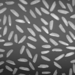
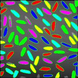
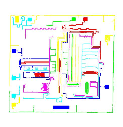
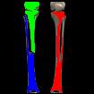
The next version of Pixcavator is to be relased in a few weeks. A new feature that I want to preview is Coloring Objects. Once objects are found, you can do anything with them. So, it was easy to implement (the objects are colored randomly). And it’s definitely an amusing feature. It can also be helpful.
This tool can help you confirm that your image segmentation is correct:
A more intricate segmentation:
Coloring combined with background removal:
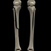
Something more amusing: recoloring objects and discovering a broken bone:
Just for fun:
For more examples, see our Image Gallery.
June 8, 2008
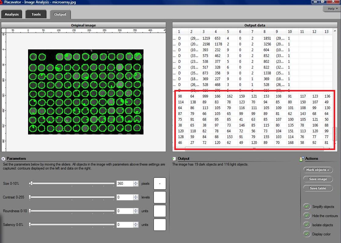
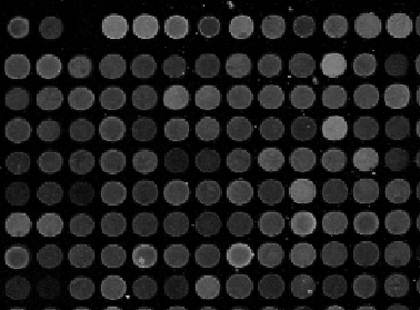 Microarrays (microplates etc) are plastic rectangles with a grid of “wells” containing biological materials. When another biological or chemical substance is added to these cells, the reaction is captured in digital images. For example, various concentrations of a chemical or a drug are added to the wells containing biological cells. The cells then start to divide faster, or slower, or simply die. The result affects the color of the substance in each cell. The image analysis automatically captures this data and draws conclusions. For example, you can pinpoint exactly at what concentration the drug becomes toxic. It’s like hundreds experiments in one! Appropriately, this is also called high throughput screening. Microarrays (microplates etc) are plastic rectangles with a grid of “wells” containing biological materials. When another biological or chemical substance is added to these cells, the reaction is captured in digital images. For example, various concentrations of a chemical or a drug are added to the wells containing biological cells. The cells then start to divide faster, or slower, or simply die. The result affects the color of the substance in each cell. The image analysis automatically captures this data and draws conclusions. For example, you can pinpoint exactly at what concentration the drug becomes toxic. It’s like hundreds experiments in one! Appropriately, this is also called high throughput screening.
I’ve been working on a related project for one of our clients and I would like to present a modified version of Pixcavator. First it captures all the wells in the form of a list with all the data about them – in the usual way. Then it displays the gray level (intensity) for each well – according to its position in the microarray. Of course, instead of intensity you can display other characteristics of these objects: the average intensity, or the standard deviation, or the average color (for color images), etc.
The point of the post is this: the hard part of collecting the data about the objects is taken care of by Pixcavator - the rest is a easy exercise with the Pixcavator SDK.
May 6, 2008
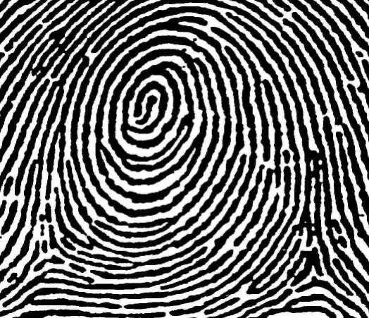
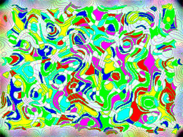
I’ve tried a variety of images and, as the diagram indicates, the processing time appears to depend linearly on the number N of pixels in the image. Roughly, 40 seconds for each million pixels in the image. The testing was done on HP Pavilion laptop with Intel Core 2 Dual CPU T7500 2.2GHz.
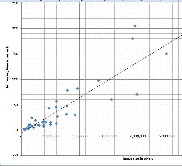
I can’t improve my estimate though. It’s O(N^2) (link to the article in Wikipedia). That’s how we get it. The analysis algorithm works as follows: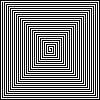
- Each pixel is processed separately.
- For each of the N pixels an object is created and you may have to run around it to mark its edges.
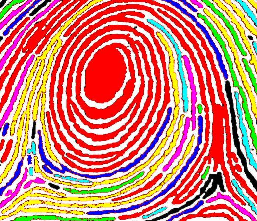
- If this object is very thin and fills the image (like this spiral), its perimeter is proportional to N.
My feeling is that the images of this kind are unusual. Maps may be close, as well as microchips, or anything fractal-like. Cells are OK.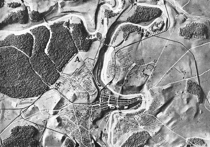 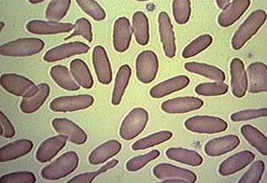
Update: The estimate O(N^2) refers to the time of image analysis - creation of the graph. After that, you still have to run up and down this graph to come up with the output data. BTW, the size of the graph and, therefore, the memory depends linearly on N, O(N).
April 29, 2008
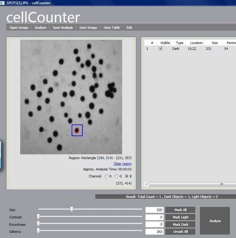
The next release of cellAnalyst due in May will have one especially nice feature. The hardest part new users find about getting the best from cellAnalyst (and Pixcavator) is discovering good analysis settings - size, contrast etc. Trial and error takes too long, expecially for larger images. Now the user will have the ability to analyze a small rectangle to find the measurements of objects - cells - he is interested in and then apply these settings for the analysis of the whole image. In more detail, this is described in the wiki under Analysis Strategy.
April 1, 2008
I decided to rename the wiki, from “Computer Vision Wiki” to “Computer Vision Primer”. “Wiki” is just such a general (and generic) term that it is easy to confuse our wiki with other wikis related to computer vision. The word “primer” helps to make a point about what makes ours different – we focus on the fundamentals and try to keep it very accessible. CVprimer.com is also easy to remember. Finally, when I get to turn this into a book, Computer Vision Primer will be a good title.
There have been some additions to the wiki. I did quite a lot of editing throughout, for example, Overview. I started to add articles on measurements of objects: saliency, mass, average contrast, diameter, minor and major axes, Euler number, Robustness of geometry and topology. Those are still quite thin. In article Machine learning in computer vision I summarized the recent blog posts on the subject. There are also many red links – those are articles I plan to write.
Pixcavator PE (photo editing) is to be released in just a few weeks. It is a simplified version of the image analysis version but it will also have a couple of new features. These features and many more will appear in Pixcavator 2.5.
cellAnalyst has now an online counterpart. You can upload your images, analyze them, save the data, and search images - all in your browser. Create your free account here. Feedback will be appreciated… Meanwhile, AssaySoft has been incorporated.
March 4, 2008
In the last post I provided a list that compared the capabilities of ImageJ (without plug-ins) and Pixcavator 2.4 in analysis of gray scale images. Then I submitted the link to the ImageJ’s forum.
The premise was very simple. The list contained enough features of ImageJ’s to show that they are comparable (in a certain narrow sense). It also contained some Pixcavator’s features that ImageJ doesn’t have to make the comparison interesting. I expected people to try it and give me some feedback. This is done every day because it’s a fair trade: people get to try something new and I get to learn something new. That didn’t happen.
My post was taken as an attack on ImageJ. The responses were along these lines:
- ImageJ is free (as in “free speech” as I was explained).
- ImageJ works on all platforms not just Windows.
- ImageJ’s plug-ins include “particle tracking, deconvolution, fourier transform, FRET analysis, 3D reconstruction, neuron tracing…”
Clearly, this wasn’t the kind of feedback I expected. I thought they were simply off topic.
To resolve the issue somewhat I added the first two items to the table and also promised to have a post to compare ImageJ with plug-ins to Pixcavator SDK (it’s free but unlike free speech it will only stay free for some time…).
Even though this was very unsatisfying, it wasn’t all bad - there were a few positive/neutral responses (thanks!) and there were spikes in the number of visits and downloads.
In retrospect, I should have made it clear that the comparison was from the point of view of a user not a developer. In this light, the main advantage of Pixcavator becomes evident – its simplicity!
So I didn’t learn anything new and didn’t get to improve my software, so what? I can turn this around and say that the end result is in fact a good news:
None of the statements in the post has been refuted.
The only statement that has been refuted – multiple times – is: “Pixcavator is better than ImageJ”, the statement I never made or implied.
One interesting reaction came from Mark Burge: “I would hazard to say that everything in Pixcavator is surely available through a plugin”. I wagered $100 that he was wrong. No response so far. How about we make this a bit more interesting? Here’s is a challenge:
$300 for the first person who shows that all of these features of Pixcavator’s are reproducible by the existing ImageJ’s plug-ins!
Meanwhile life goes on. We had a couple of milestones recently. First, we reached 30,000 downloads of Pixcavator since January 2007 (versions 2.2 – 2.4). Second, the wiki - the main page – has been visited 10,000 times since August 2007. Recently we are getting over 80 daily visitors.
January 21, 2008
These are the highlights and random thoughts.
- Santa Barbara: ocean on one side, mountains on the other, and 65 degrees! In 3 days I didn’t see a single cloud. The sky was so blue that it looked photoshopped.

- The workshop was very well organized. The only problem I had was that you didn’t get a break after every talk. You need 5 minutes to digest, recharge, discuss the talk with your neighbor, or just stretch your legs.
- The talks were mostly academic (zebra fish is pretty much covered). But 3-4 talks were excellently presented and very educational.
- This biology stuff is complicated!
- Most image analysis methods are intended for specific problems. But, in addition, each problem may have different methods eqully applicable. No-one is concerned that the results could be also different (see last post).
- The Open Microscopy Environment could have a good future.
- One non-academic talk was by a person from Definiens. Unfortunately only generalities were presented followed by a few examples. Secretive. A top-down approach isn’t a good idea anyway.
- Dr. Pahwa and I had a few good discussions about cellAnalyst with several people. More in a couple of days.

- You get 65 degrees only for a few hours in the afternoon. When you get out in the morning, it’s more like 40 or less.
December 14, 2007
The extended abstract of the presentation is here - PDF. It will be given at Workshop on Bio-Image Informatics: Biological Imaging, Computer Vision and Data Mining, 2008, Center for Bio-Image Informatics, UCSB, Santa Barbara, CA, USA, January 17-18, 2008. We will be testing cellAnalyst now. More updates to come.
BTW, counting objects is by its nature a topological issue. So, from the topological point of view there shouldn’t the word ‘topological’ in the title!
Update: cellAnalyst can be downloaded at cellAnalyst.net.
December 5, 2007
A few recent developments:
The number of downloads of Pixcavator 2.3 has reached 10,000.
Idee has re-launched its visual image search application. There is no image uploading and as a result no way to test it. But even sSearching within its own collection of images indicates that shapes aren’t given serious consideration. More on image search here. More updates to come.
Last Sunday Ash Pahwa and I attended the exhibit of the annual meeting of the American Society for Cell Biology in Washington DC. We talked with some companies that make image analysis and related software. Nothing spectacular. Most interesting was the conversation with Ilya Goldberg, the representative of OME (Open Microscopy Environment).
A quick analysis revealed that the time complexity of the image analysis algorithm that runs Pixcavator is O(n2), where n is the number of pixels in the image.
November 19, 2007
Dr. Ash Pahwa and I will give a presentation at Workshop on Bio-Image Informatics: Biological Imaging, Computer Vision and Data Mining, 2008, Center for Bio-Image Informatics, UCSB, Santa Barbara, CA, USA, January 17-18, 2008. The abstract is below.
A Topological Approach to Cell Counting
Peter Saveliev (Marshall University, Huntington, WV) and Ash Pahwa (Mayachitra Inc., Santa Barbara, CA)
Cell counting and identification is a common task in biology and pathology. To automate this task one has to approach it as an image segmentation problem. Many researchers have solved this problem following various strategies. The approach we propose relies on topology, which is the science of continuity and connectedness that studies spatial relations within the image. An image pixel is defined to have 4 vertices (corners), 4 edges, and one face. Algebraic topology uses algebraic operations with these objects to count the number of completed cycles – circular sequences of edges. The completion of a cycle indicates the presence of a cell. In the case of gray scale, our strategy for counting cells is to count dark objects with light background and light objects with dark background. The types of images our algorithm is most suitable for are those that represent something 2-dimensional (rather than 2D images of 3D objects) such as images of cellular tissue or blood cells under a microscope.
The topological nature of the algorithm makes it especially suitable for cell counting. First, the count of cells is independent of their locations. Second, the measurements of cells are independent of their orientations with respect to the image grid. Third, the algorithm captures cells and other features regardless of their sizes, shapes, and locations with no deformation, smoothing, blurring or approximation.
We developed a software suite called cellAnalyst with the following output: the image with cells’ contours captured and a spreadsheet with cells’ locations and characteristics such as area, perimeter, intensity, and contrast. The processing starts with an automatic analysis of the image that produces a graph that contains complete data about the image. The user proceeds in a semiautomatic mode to interactively visualize various segmentations. By moving sliders corresponding to cells’ characteristics the user instantly changes the cells’ boundaries and can choose the most appropriate segmentation. The output data is then updated in real time. The user can also exclude noise and irrelevant details from the analysis by simply clicking on them.
The analysis data has been verified using pathology and retinal images. The images are analyzed by manually counting, identifying, and measuring cells and the results are compared with the output of cellAnalyst. The matches have been reliable and repeatable.

— Next Page » |
|
|


")


