According the ImageJ site: “Watershed segmentation is a way of automatically separating or cutting apart particles that touch”.

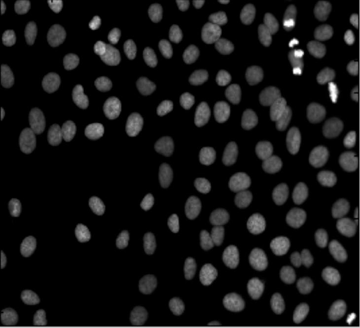
Suppose black is the particles and white is the background. The the procedure is fairly simple.

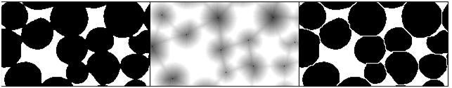
First, for each pixel compute the distance to the nearest white pixel. This is called the distance function. It’s a scalar function of two variables.

Next, find the maximum points of this function. Each of these pixels will become the center of a particle.

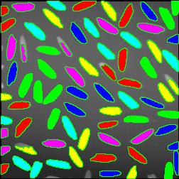
You carry out multiple rounds of dilation that gradually grow these particles. The dilation has two restrictions. First, the particles aren’t allowed to grow beyond the original set of black pixels. This way we guarantee that we end up with the same set of pixels except it has been “cut” into pieces. Second, a new pixel isn’t added if it’s adjacent to a pixel that belongs to another particle. This way the particles start to “push” onto each other but never overlap.

The tricky part of the last restriction is that the growth rate will have to be different for particles of different sizes. Otherwise, two particles will always be separated by a cut exactly half way between their centers. That wouldn’t make sense if one is significantly larger than the other. Roughly, the dilation rate should be proportional to the value of the distance function.

Some questions remain. For example, how does one efficiently find the maxima? Everything is discrete, so forget about partial derivatives etc. You have to visit every point.

How does one deal with particles that are simply noise? If you remove all small particles, you may have nothing left. One answer is to discard the maxima with low values of the distance function.

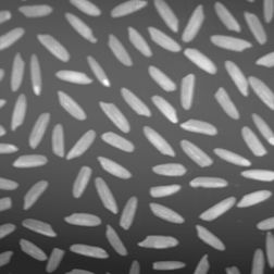
Another issue is typical for many image analysis techniques. Once again to quote the ImageJ site, “Watershed segmentation works best for smooth convex objects that don’t overlap too much.” Basically, you have to view (analyze!) the image yourself and decide ahead of time whether the method is appropriate. There is a good reason to be cautious – non-convex particles may cause the watershed method to produce undesirable results.

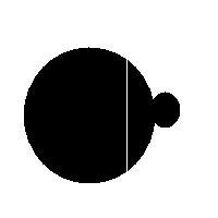
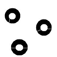
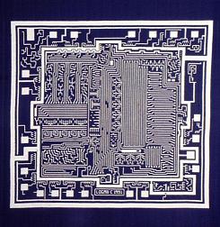
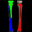
You have to choose ahead of time whether you have white or black particles. If you don’t do it correctly, you end up with non-convex black “particles”. The result of watershed segmentation isn’t what you expect:

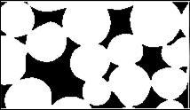
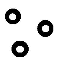
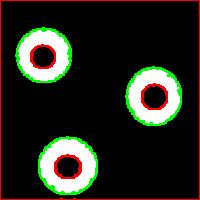
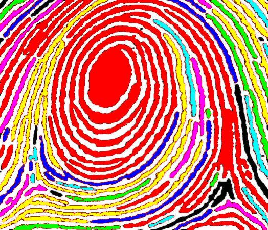
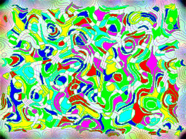
It is also easy to think of an image (rings) that can’t possibly be analyzed correctly by watershed regardless of the black/white choice:

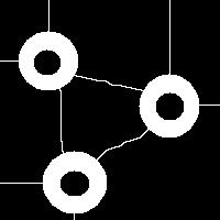
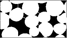
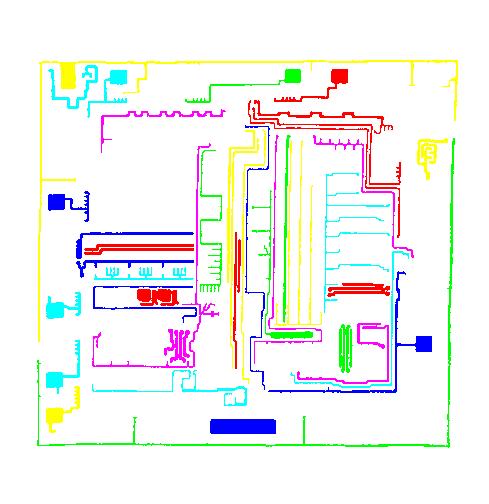
Needless to say that the topological method produces the correct segmentation here:

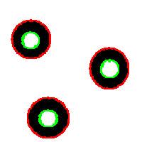
It can’t however separate particles yet (the stuff will appear in the wiki under Robustness of topology).

The next version of Pixcavator is to be relased in a few weeks. A new feature that I want to preview is Coloring Objects. Once objects are found, you can do anything with them. So, it was easy to implement (the objects are colored randomly). And it’s definitely an amusing feature. It can also be helpful.

This tool can help you confirm that your image segmentation is correct:

A more intricate segmentation:

Coloring combined with background removal:

Something more amusing: recoloring objects and discovering a broken bone:

Just for fun:

For more examples, see our Image Gallery.

Let’s go to Wikipedia. The first sentence is:

“Image segmentation is partitioning a digital image into multiple regions”.

This description isn’t what I would call a definition as it suffers from a few very serious flaws.

First, what does “partitioning” mean? A partition is a representation of something as the union of non-overlapping pieces. Then partitioning is a way of obtaining a partition. The part about the regions not overlapping each other is missing elsewhere in the article: “The result of image segmentation is a set of regions that collectively cover the entire image” (second paragraph).

Then, is image segmentation a process (partitioning) or the output of that process? The description clearly suggests the former. That’s a problem because it emphasizes “how” over “what”. That suggests human involvement in the process that is supposed to be objective and reproducible.

Next, a segmentation is a result of partitioning but not every partitioning results in a segmentation. A segmentation is supposed to have something to do with the content of the image.

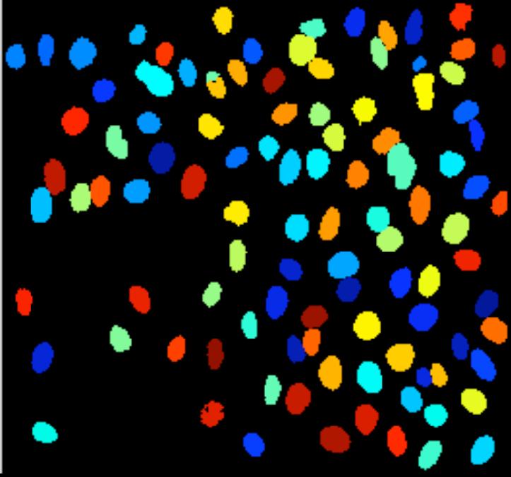More nitpicking. Do the regions have to be “multiple”? The image may be blank or contain a single object. Does the image has to be “digital”? Segmentation of analogue images makes perfect sense.

A slightly better “definition” I could suggest is this:

A segmentation of an image is a partition of the image that reveals some of its content.

This is far from perfect. First, strictly speaking, what we partition isn’t the image but what’s often called its “carrier” – the rectangle itself. Also, the background is a very special element of the partition. It shouldn’t count as an object…

Another issue is with the output of the analysis. The third sentence is “Image segmentation is typically used to locate objects and boundaries (lines, curves, etc.) in images.” It is clear that “boundaries” should be read “their boundaries” here - boundaries of the objects. The image does not contain boundaries – it contains objects and objects have boundaries. (A boundary without an object is like Cheshire Cat’s grin.)

Once the object is found, finding its boundary is an easy exercise. This does not work the other way around. The article says: “The result of image segmentation [may be] a set of contours extracted from the image.” But contours are simply level curves of some function. They don’t have to be closed (like a circle). If a curve isn’t closed, it does not enclose anything – it’s a boundary without an object! More generally, searching for boundaries instead of objects is called “edge detection”. In the presence of noise, one ends up with just a bunch of pixels – not even curves… And by the way, the language of “contours”, “edges”, etc limits you to 2D images. Segmentation of 3D images is out of the window?

I plan to write a few posts about specific image segmentation methods in the coming weeks.

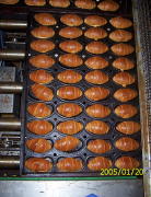
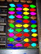
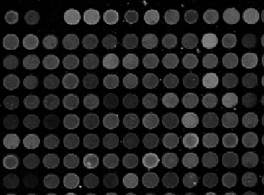Microarrays (microplates etc) are plastic rectangles with a grid of “wells” containing biological materials. When another biological or chemical substance is added to these cells, the reaction is captured in digital images. For example, various concentrations of a chemical or a drug are added to the wells containing biological cells. The cells then start to divide faster, or slower, or simply die. The result affects the color of the substance in each cell. The image analysis automatically captures this data and draws conclusions. For example, you can pinpoint exactly at what concentration the drug becomes toxic. It’s like hundreds experiments in one! 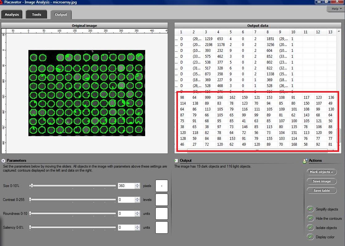Appropriately, this is also called high throughput screening.

I’ve been working on a related project for one of our clients and I would like to present a modified version of Pixcavator. First it captures all the wells in the form of a list with all the data about them – in the usual way. Then it displays the gray level (intensity) for each well – according to its position in the microarray. Of course, instead of intensity you can display other characteristics of these objects: the average intensity, or the standard deviation, or the average color (for color images), etc.

The point of the post is this: the hard part of collecting the data about the objects is taken care of by Pixcavator - the rest is a easy exercise with the Pixcavator SDK.

In part 1 and part 2 I discussed a paper on face recognition and the methods it relies on. Recall, each 100×100 gray scale image is a table of 100×100 = 10,000 numbers that can be rearranged into a 10,000-vector or a point in the 10,000-dimensional Euclidean space. As we discovered in part 2, using the closedness of these points as a measurement of similarity between images ignores the way the pixels are attached to each other. A deeper problem is that unless the two images are aligned first, there is no way to use this representation to discover that they depict the same or similar thing. The proper term for this alignment is image registration.

The similarity between images represented this way will be entirely based on their overlap. As result, the distance can be large even between images that we would consider similar. In part 2 we had examples of one-pixel images. More realistic examples are these:

• image with an object in one corner onewith the same object in another corner;
• image of a cross and the same cross turned 45 degrees;
• etc.

Back to face identification. As the faces are points in the 10,000-dimensional space, these points should be grouped somehow. The point is that all images of the same individual should belong to one group and not any other. It is common to consider “clusters” of points, i.e., groups formed of point close to each other. This was discussed above.

Now, in this paper the approach is different: a new point (the face to be identified) is represented as a linear combination of all other points (all faces in the collection).

As we know from linear algebra, this implies the following. (1) the entire collection has to be linearly dependent, (2) you can find a subcollection that adds up to 0! In other words, everything cancels out and you end up with a blank photo. Is it possible? If the dimension is low or the collection is large (the images are small relative to the number of images), maybe. What if the collection is small? (It is small – see below.) It seems unlikely. Why do I think so? Consider this very extreme case: you may need the negative for each face to cancel it: same shape with dark vs. light hair, skin, eyes, teeth (!).…

Second, the new image in the collection has to be a linear combination of training images of the same person. In other words, any image of person A is represented as a linear combination of other images of A in the collection, ideally. (More likely this image is supposed to be closer to the linear space spanned by these images.) The approach could only work under the assumption that people are linearly independent:

No face in the collection can be represented as a linear combination of the rest of the faces.

It’s a bold assumption.

If it is true, then the challenge is to make the algorithm efficient enough. The idea is that you don’t need all of those pixels/features and they in fact could be random. That must be the point of the paper.

The testing was done on two collections with several thousand images each. That sounds OK, but the number of individuals in these collections was 38 and 114!

To summarize, there is nothing wrong with the theory but its assumptions are unproven and the results are untested.

P.S. It’s strange but after so many years computer vision still looks like an academic discipline and not an industry.