August 31, 2008
I recently got a new book to read, From Gestalt Theory to Image Analysis, A Probabilistic Approach by Desolneux, Moisan, and Morel. I’ve heard of Gestalt before – apparently it’s a psychology theory of the mind. There is also an image analysis angle as Gestalt is a German word for “form” or “shape”. In the introduction the book presents are few Gestalt principles and gives them a mathematical interpretation. One principle I found especially relevant.
Werthheimer’s contrast invariance principle: Image interpretation does not depend on actual values of the gray levels, but only their relative values.
As the book further explains, the principle comes from the fact that one shouldn’t expect or rely on precise measurements of intensity. Once again this is our example:
 
The second part of the principle suggests that one should look at the level sets of the gray scale function, as well as sub- and supra-level sets. In the blurred image above, the circle is still recognizable regardless of the low contrast. Which should be picked to evaluate the size of the circle is ambiguous however.
So far, so good. Unfortunately, next the authors concentrate on supra-level (or “upper level”) sets exclusively. This is a common approach. The result is that you recognize only light objects on dark background. To see dark on light will take an extra step (invert colors). Meanwhile the case of objects with holes (or dark spots on light objects) becomes really messy. Our algorithm builds the hierarchy of dark and- light objects in one sweep (see Topology graph).
The book isn’t really about Werthheimer’s principle but another one (more of a definition).
Helmholtz principle: Gestalts are sets of points whose (geometric regular) special arrangements could not occur in noise.
This should be interesting…
August 24, 2008
Previously we discussed the watershed algorithm for binary images. One thing that wasn’t explained was where the name comes from.
We start with the following approach. According to Gonzales and Woods: “we think of a gray scale image as a topological surface, where the values of f(x,y) are interpreted as heights.” This is good (except the redundant “topological”) and quite clear. Mathematically, if f(x,y) gives the value of gray of the pixel (x,y), we simply end up with the -graph of f (remember precalc?).
Next, we find the “catchment” basins. Mathematically, these are minimum points of the surface. However, to find basins’ borders we need to find the ridge lines that separate them. Mathematically, those are lines that go from one maximum point to another via the saddle points.
To summarize, we create a surface from the image by using the value of gray at a given pixel as the height of the surface above it. The light areas are the peaks and the dark areas are the valleys. Next, we flood the valleys, gradually. As we do that, we don’t allow the water to flow from one valley to another. How? By building dams. These dams will break the image into regions each containing a single valley. That’s image segmentation.
Let’s now take a look at the Wikipedia article: “The watershed algorithm is an image processing segmentation algorithm that splits an image into areas, based on the topology of the image.” First, any segmentation algorithm splits an image into areas. Second, any segmentation should be based on the topology of the image. So, what’s left is “The watershed is an image segmentation algorithm”.
The next sentence is “The length of the gradients is interpreted as elevation information.” Wait a minute, that’s not the same! The length of the gradient is the steepness of the surface. In the next sentence however the article seems comes back to the standard approach: “During the successive flooding of the grey value relief, watersheds with adjacent catchment basins are constructed.” And then again: “This flooding process is performed on the gradient image…” Using the gradient as the surface is an alternative approach to the watershed, so this must be a mix-up. Another approach is using the distance function for binary images.
We’ll discuss these issues in the next post.
August 20, 2008
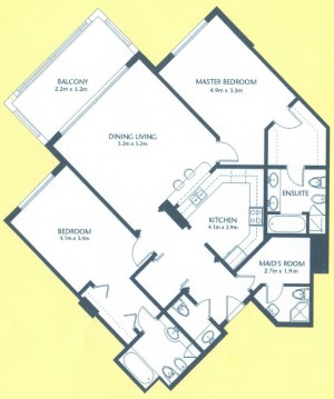 As a suggestion from one of our users, we used Pixcavator to analyze floorplans. The task is very simple – measure the rooms. As a suggestion from one of our users, we used Pixcavator to analyze floorplans. The task is very simple – measure the rooms.
Measuring irregular (or even regular) isn’t easy for a person because unless all rooms are rectangular one needs know some geometry. If the corners aren’t 90 degrees, you may have to measure them and then (OMG!) use trigonometry. The walls can also be curved. If the curves are known, all you need is calculus (OMG!!). It is unlikely that the formulas for the curves come with the floorplan, so digital image analysis seems inevitable.
The results are below. Of course, I had to “close” the doors first.
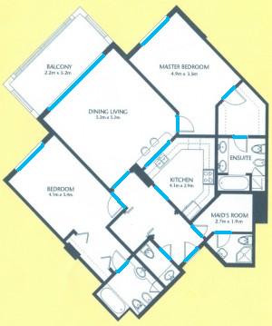 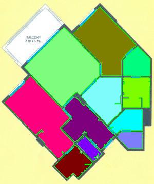
Calbration wasn’t addressed though.
August 10, 2008
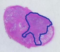
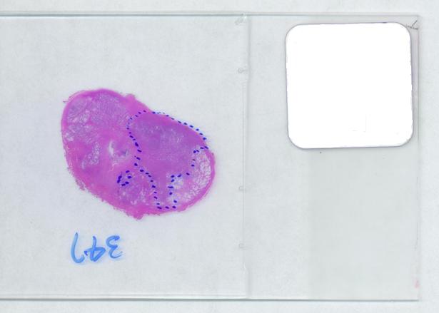 The first picture explains what normally happens when a prostate tumor has to be evaluated. The prostate is cut into thin slices and the slices are put on pieces of glass. Next, the doctor outlines the tumor within the prostate with a marker. Finally, the area of the outlined region is evaluated in each slice and the volume of the tumor is estimated. The first picture explains what normally happens when a prostate tumor has to be evaluated. The prostate is cut into thin slices and the slices are put on pieces of glass. Next, the doctor outlines the tumor within the prostate with a marker. Finally, the area of the outlined region is evaluated in each slice and the volume of the tumor is estimated.
Evaluating the area of the tumor with a naked eye will give you a very low accuracy. Best one can do to improve that is to superimpose a grid over the image and count the number of squares that fall into the tumor. Then the accuracy will be inversly proportional to the size of the square but the smaller the square the more complex the manual counting will be.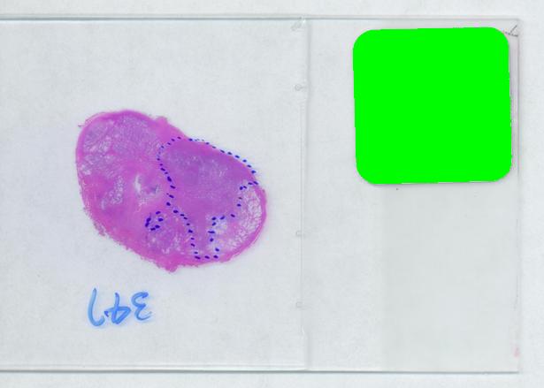
Digital image analysis is a necessity here.
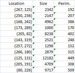
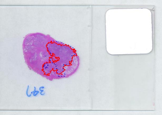
I analyzed the shrunk version (615×439) of the image with Pixcavator followed by some back-of-the-envelope calculations.
The critical part of analysis is the calibration. For that I used the square label in the image. It is known that its side is 2.2 cm. Now, I pushed the size slider almost all the way to the right and ended up with just one object -the label (green). Its area according to the table is 29,516 pixels. If we ignore the round corners (introducing some error here, unfortunately), it is a square. So 29,810 pixels = 2.2 * 2.2 = 4.84 sq cm.
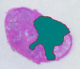
Next, the tumor. The dotted line is made solid using MS Paint. The you run Pixcavator. The contour has the area of 9,491 pixels. So, it is 9,491 * 4.84 / 29,810 = 1.54 sq cm.
 The end. The end.
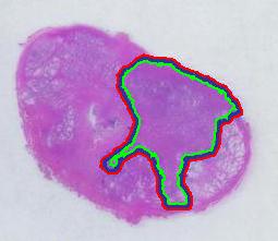
There is still the issue of error however. The error produced by hand drawing is estimated in the next experiment. Pixcavator evaluated the area on the outside of the curve (9,774) and on the inside (7,112). Hence the area of the curve is (9,774– 7,112) / 9,774 = 27% of the outside of the tumor. That’s the error.
It seems too high!
To verify the result, let’s approach from another direction. The perimeters are 542 and 530 respectively. Then the average thickness of the line is (9840-7342)/536 = 4.7 pixels. Examination of the image confirms this number. Of course, the error can be easily cut down by making the line 1/2 thinner but it will still remain high…
That brings us to the possibility of discovering the tumor within the prostate automatically. To be precise, the procedure would be semi-automatic not automatic, and it is the doctor who would make all the decisions. He chooses the contours and Pixcavator just counts pixels. What it gives you is a procedure that is somewhat simple – moving sliders until you have a good fit – and quite accurate – if the fit is good. Finding a good contour won’t require training but just a bit of practice. The last image shows that this approach isn’t totally unreasonable…
August 3, 2008
Image analysis and computer vision is the extraction of meaningful information from digital images. One of the most prominent application of computer vision is in medical image processing - extraction of information for the purpose of making a medical diagnosis. It can be detection and measurement of tumors, arteriosclerosis or other malign changes or it can be identifying and counting cells, etc. Other main areas are industrial machine vision (automatic quality inspection, robotics, etc) and the military (missile guidance, battlefield awareness, etc).
The science of computer vision consists of an abundance of image analysis methods. These methods have been developed over the years for solving various but often narrow image analysis tasks. The result is that these methods are very task specific and seldom can be applied to a broad range of applications.
Our conclusion is then that as a discipline computer vision lacks a solid mathematical foundation.
Our long term goal is to design a comprehensive computer vision system “from first principles”. These principles come initially from one of the most fundamental fields of mathematics, topology. The idea is that just as mathematics rests on topology (and algebra), computer vision should be built on a firm topological foundation.
Algebraic topology is a well established discipline within mathematics. Its main computational tools have been implemented as software (CHomP, Computational Homology Project, and others). However, this theory and these tools are only applicable to binary images.
A framework for analysis of gray scale images has been under development. It is called Pixcavator. It includes both an image analysis software and an SDK. Pixcavator was into a product that also includes image management and database capabilities.
Some further issues remain. Future projects include the development of:
- protocols for applying the framework for specific tasks (e.g., tumor measurement),
- new methods that resolve the ambiguity of the boundaries of objects in gray scale images,
- integration of the existing image analysis methods into the framework,
- a framework for video (first binary, then gray scale, etc),
- a framework for color images (and other multichannel images),
- a framework for 3D images (first binary, then gray scale, etc).
July 29, 2008
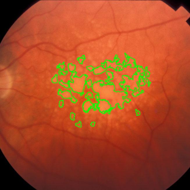
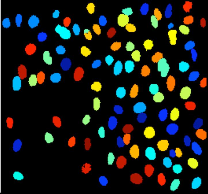
During a retina inspection one of the most common pathology is Drusen deposits. Some computer assisted methods have been created to solve this problem and especially avoid the subjectivity of the doctors (”MD3RI a Tool for Computer-Aided Drusens Contour Drawing”) [1].
An image from this paper is below:
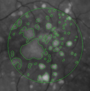
Pixcavator easily produces similar results:
Another example is ice cracking (thanks to Nikolay Makarenko for the idea). The image is analyzed with Pixcavator with settings 596-63.
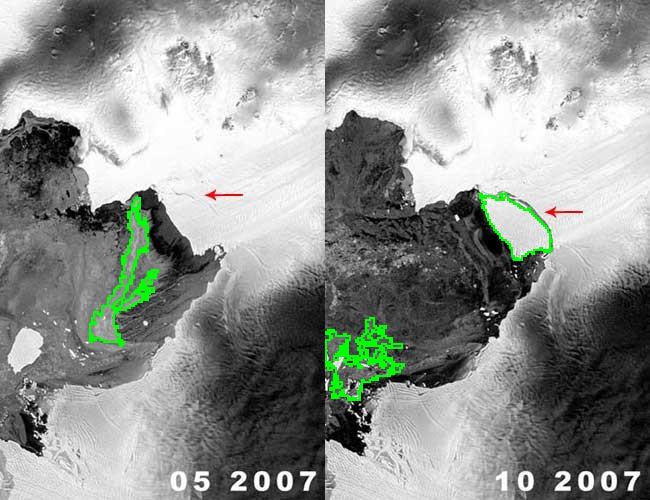
An iceberg is born!
These kind of examples will appear in the wiki under Case studies.
July 27, 2008
The paper (PDF, 10 pages, 360K) describes the algorithm behind Pixcavator. The algorithm is presented in detail in the wiki but this is a new and improved exposition. I reconsidered some of the terminology, re-wrote the pseudocode, and improved illustrations. There is also a gap in the wiki - when an edge is added to the image, case 4 is missing. I’ll have to re-write a few articles. The presentation in the paper is less detailed (in terms of examples, images etc) but it is a bit more thorough.
Abstract: The paper provides a method of image segmentation of binary and gray scale images. For binary images, the method captures not only connected components but also the holes. For gray scale images, there are two kinds of “connected components” – dark regions surrounded by lighter areas or light regions surrounded by darker areas.
The long term goal is to design a computer vision system “from first principles”. The last sentence in the abstract is one such principle. Keep in mind (of course) that if every dark region surrounded by a lighter area is an object, it does not mean that every object is a dark region surrounded by a lighter area (or vice versa). In a way, these are “potential” objects and you still have to filter and/or group them to find the “real” ones. So there must be more first principles.
The paper does not go far beyond this stage. The main step is – all potential objects are recorded in the “topology graph” (“frame graph” in the wiki). Then only one method of filtering is presented (the one based on size).
All feedback is welcome.
July 20, 2008
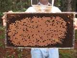 This came as a question from one of our users. The picture explains the problem: there is a bee frame with several hundred sealed brood. They are visible as tan hexagons (the dark circles are empty cells). Now, count them! Just like that – an outdoors photo taken with a regular digital camera, no registration, no calibration, etc. This came as a question from one of our users. The picture explains the problem: there is a bee frame with several hundred sealed brood. They are visible as tan hexagons (the dark circles are empty cells). Now, count them! Just like that – an outdoors photo taken with a regular digital camera, no registration, no calibration, etc.
The problem is interesting but also quite challenging. The sealed cells aren’t separated enough from each other to count them one by one with 100% accuracy. For that 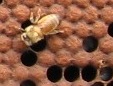 the image would need a higher resolution. If, however, the goal is just an estimate, Pixcavator can help. Then the task is less about counting and more about measuring… and some elementary school math. the image would need a higher resolution. If, however, the goal is just an estimate, Pixcavator can help. Then the task is less about counting and more about measuring… and some elementary school math.
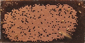
First I cropped the image. Then I analyzed it with 100-130 settings, no shrinking. The result is 311 dark objects (clusters of empty cells) with the average size 1,255. So the total area of the empty cells is
311*1,255 = 390,305.
Since the image is 1,394×709, the area covered by sealed cells is
1,394*709 - 390,305 = 598,041.
 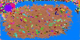
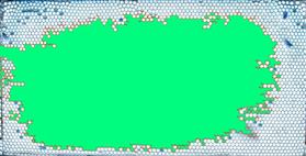
Just in case I decided to validate this number from another source. I analyzed the negative with 100-110 settings. Then I just picked the largest object in the table - the cluster of all sealed cells. Its area is 613,814. Since the empty cells inside of this area aren’t taken into account, the result is higher than the first estimate. The difference is however less than 3%.
At this point you need to estimate the size of a cell. Looking at a few individual cells in the table may give you an estimate, but it would take some work with Excel. Instead I did actual measuring - on the screen. I counted 10 cells in a row and measured the length with a ruler - 34 mm. So each cell is about 3.4×3.4 mm. Next I measured the image - 270×136 mm. So the number of cells is
270*136/(3.4*3.4) = 36,720.
(The user won’t need this computation because the actual number is known). Then the size of the cell is
(the size of the image in pixels) / (the number of cells) = 1,394*709/36,720 = 269.
Finally, the number of sealed cells is
(the total area) / (the size of each) = 598,041/269 = 2,223.
The hand counted number is 2,198. The error is about 1%!
You can reproduce these results with Pixcavator version 3.0 or earlier and this full size image: http://inperc.com/wiki/images/7/7d/Bee_brood-cropped.jpg.
July 13, 2008
On several occasions I was asked: Why wouldn’t we add a second slider to the size ruler? The logic is very convincing: “the first slider removes objects from analysis that are too small - with the second slider you can exclude objects that are too large”. There are real life problems that need this kind of analysis.
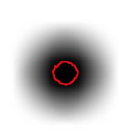
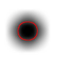
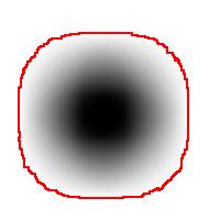
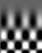
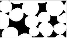
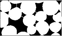
What is wrong with this idea? The problem is that the idea is “binary”. If the image is binary, excluding larger objects is a simple operation. We however deal with gray scale images. Sometimes objects in gray scale images look just like ones in binary images but often they have no well defined boundary. No well defined boundary – no well defined size!
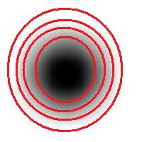
For example, this is a binary image of a circle and that is the same image blurred. There is clearly just one object here and it looks like circle. But what’s its size? It could be a small spot in the middle, or large circle, or it could be the whole image (why not?). If there are several objects like that, we can’t filter them based on larger/smaller comparison. As a result, we can’t even count them properly because without measuring we can’t tell noise from what’s important.
But wait a minute, of course, our software counts objects! So, how?
The user sets a lower bound on sizes of objects he considers important. Anything smaller is noise. What the user doesn’t know (but should) is what is an object. The definition of an object is in fact very simple:
An object is either a dark region surrounded by lighter area or a light region surrounded by a darker area.
For example, in the above image we have many-many circular objects. Too many, in fact, because we know that there is only one! So, the objects that we’ve found aren’t actual objects but “potential” objects. At this point we need to select just one. How?
We use the bound chosen by the user! We exclude all potential objects that are smaller than this bound. Good, but even now we still have multiple objects. What do we do? We just take the smallest!
 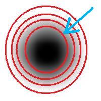
Roughly, once the bound is set, the object is allowed to grow until its size is over the bound.
Suppose the bound is 100. Then what we present as the output is objects larger than 100 BUT as close as possible to 100. If the gray level changes very gradually, the objects’ sizes end up almost exactly equal 100. If this is the case, having an upper bound (say 200) in addition to the lower bound would not change the outcome…
That’s why only a single slider for the size is present. If object A is larger than object B, A is at least as important as B. A priori, all things being equal.
The second slider is for contrast and it operates in the exact same way: the object is allowed to grow until its contrast is over the bound. The logic is the same as before: a priori, if object A has a higher contrast than object B, A is at least as important as B.
OK, but what about those real life situations when you need to exclude larger objects? That’s when you turn from image analysis to data analysis. Of course, you’d have to make sure that you have captured all objects that you care about. That’s the hard part.
The data analysis stage is the easy part. If you have captured some noise or objects that you want to exclude, that’s OK. Now you simply filter the objects on the list based on any characteristic you want. Excel has plenty of tools for that. For example, the size is too large or too small. Or the perimeter, the contrast, the roundness, the intensity. Maybe you want only the objects from 100 to 200 pixels in size. Or maybe you are only interested in the objects within 300 pixels from the center of the image. All is easy at this stage.
June 29, 2008
According the ImageJ site: “Watershed segmentation is a way of automatically separating or cutting apart particles that touch”.
Suppose black is the particles and white is the background. The the procedure is fairly simple.
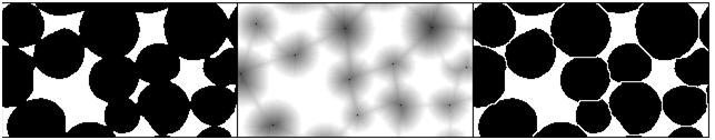
First, for each pixel compute the distance to the nearest white pixel. This is called the distance function. It’s a scalar function of two variables.
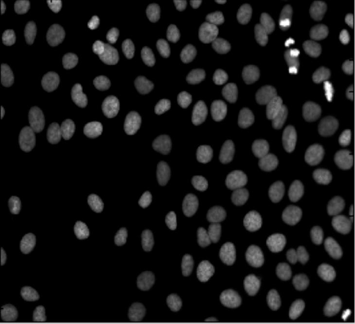
Next, find the maximum points of this function. Each of these pixels will become the center of a particle.
You carry out multiple rounds of dilation that gradually grow these particles. The dilation has two restrictions. First, the particles aren’t allowed to grow beyond the original set of black pixels. This way we guarantee that we end up with the same set of pixels except it has been “cut” into pieces. Second, a new pixel isn’t added if it’s adjacent to a pixel that belongs to another particle. This way the particles start to “push” onto each other but never overlap.
The tricky part of the last restriction is that the growth rate will have to be different for particles of different sizes. Otherwise, two particles will always be separated by a cut exactly half way between their centers. That wouldn’t make sense if one is significantly larger than the other. Roughly, the dilation rate should be proportional to the value of the distance function.
Some questions remain. For example, how does one efficiently find the maxima? Everything is discrete, so forget about partial derivatives etc. You have to visit every point.
How does one deal with particles that are simply noise? If you remove all small particles, you may have nothing left. One answer is to discard the maxima with low values of the distance function.
Another issue is typical for many image analysis techniques. Once again to quote the ImageJ site, “Watershed segmentation works best for smooth convex objects that don’t overlap too much.” Basically, you have to view (analyze!) the image yourself and decide ahead of time whether the method is appropriate. There is a good reason to be cautious – non-convex particles may cause the watershed method to produce undesirable results.
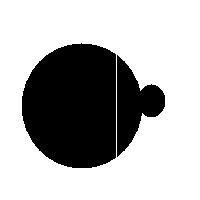
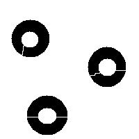
You have to choose ahead of time whether you have white or black particles. If you don’t do it correctly, you end up with non-convex black “particles”. The result of watershed segmentation isn’t what you expect:
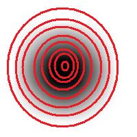
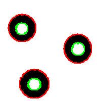
It is also easy to think of an image (rings) that can’t possibly be analyzed correctly by watershed regardless of the black/white choice:
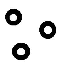  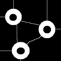
Needless to say that the topological method produces the correct segmentation here:
 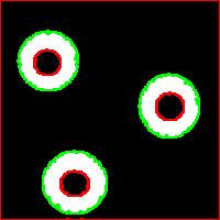
It can’t however separate particles yet (the stuff will appear in the wiki under Robustness of topology).
June 15, 2008
Let’s go to Wikipedia. The first sentence is:
“Image segmentation is partitioning a digital image into multiple regions”.
 This description isn’t what I would call a definition as it suffers from a few very serious flaws. This description isn’t what I would call a definition as it suffers from a few very serious flaws.
First, what does “partitioning” mean? A partition is a representation of something as the union of non-overlapping pieces. Then partitioning is a way of obtaining a partition. The part about the regions not overlapping each other is missing elsewhere in the article: “The result of image segmentation is a set of regions that collectively cover the entire image” (second paragraph).
Then, is image segmentation a process (partitioning) or the output of that process? The description clearly suggests the former. That’s a problem because it emphasizes “how” over “what”. That suggests human involvement in the process that is supposed to be objective and reproducible.
Next, a segmentation is a result of partitioning but not every partitioning results in a segmentation. A segmentation is supposed to have something to do with the content of the image.
 More nitpicking. Do the regions have to be “multiple”? The image may be blank or contain a single object. Does the image has to be “digital”? Segmentation of analogue images makes perfect sense. More nitpicking. Do the regions have to be “multiple”? The image may be blank or contain a single object. Does the image has to be “digital”? Segmentation of analogue images makes perfect sense.
A slightly better “definition” I could suggest is this:
A segmentation of an image is a partition of the image that reveals some of its content.
This is far from perfect. First, strictly speaking, what we partition isn’t the image but what’s often called its “carrier” – the rectangle itself. Also, the background is a very special element of the partition. It shouldn’t count as an object…
Another issue is with the output of the analysis. The third sentence is “Image segmentation is typically used to locate objects and boundaries (lines, curves, etc.) in images.” It is clear that “boundaries” should be read “their boundaries” here - boundaries of the objects. The image does not contain boundaries – it contains objects and objects have boundaries. (A boundary without an object is like Cheshire Cat’s grin.)
Once the object is found, finding its boundary is an easy exercise. This does not work the other way around. The article says: “The result of image segmentation [may be] a set of contours extracted from the image.” But contours are simply level curves of some function. They don’t have to be closed (like a circle). If a curve isn’t closed, it does not enclose anything – it’s a boundary without an object! More generally, searching for boundaries instead of objects is called “edge detection”. In the presence of noise, one ends up with just a bunch of pixels – not even curves… And by the way, the language of “contours”, “edges”, etc limits you to 2D images. Segmentation of 3D images is out of the window?
I plan to write a few posts about specific image segmentation methods in the coming weeks.
June 2, 2008
In part 1 and part 2 I discussed a paper on face recognition and the methods it relies on. Recall, each 100×100 gray scale image is a table of 100×100 = 10,000 numbers that can be rearranged into a 10,000-vector or a point in the 10,000-dimensional Euclidean space. As we discovered in part 2, using the closedness of these points as a measurement of similarity between images ignores the way the pixels are attached to each other. A deeper problem is that unless the two images are aligned first, there is no way to use this representation to discover that they depict the same or similar thing. The proper term for this alignment is image registration.
The similarity between images represented this way will be entirely based on their overlap. As result, the distance can be large even between images that we would consider similar. In part 2 we had examples of one-pixel images. More realistic examples are these:
- image with an object in one corner onewith the same object in another corner;
- image of a cross and the same cross turned 45 degrees;
- etc.
Back to face identification. As the faces are points in the 10,000-dimensional space, these points should be grouped somehow. The point is that all images of the same individual should belong to one group and not any other. It is common to consider “clusters” of points, i.e., groups formed of point close to each other. This was discussed above.
Now, in this paper the approach is different: a new point (the face to be identified) is represented as a linear combination of all other points (all faces in the collection).
As we know from linear algebra, this implies the following. (1) the entire collection has to be linearly dependent, (2) you can find a subcollection that adds up to 0! In other words, everything cancels out and you end up with a blank photo. Is it possible? If the dimension is low or the collection is large (the images are small relative to the number of images), maybe. What if the collection is small? (It is small – see below.) It seems unlikely. Why do I think so? Consider this very extreme case: you may need the negative for each face to cancel it: same shape with dark vs. light hair, skin, eyes, teeth (!).…
Second, the new image in the collection has to be a linear combination of training images of the same person. In other words, any image of person A is represented as a linear combination of other images of A in the collection, ideally. (More likely this image is supposed to be closer to the linear space spanned by these images.) The approach could only work under the assumption that people are linearly independent:
No face in the collection can be represented as a linear combination of the rest of the faces.
It’s a bold assumption.
If it is true, then the challenge is to make the algorithm efficient enough. The idea is that you don’t need all of those pixels/features and they in fact could be random. That must be the point of the paper.
The testing was done on two collections with several thousand images each. That sounds OK, but the number of individuals in these collections was 38 and 114!
To summarize, there is nothing wrong with the theory but its assumptions are unproven and the results are untested.
P.S. It’s strange but after so many years computer vision still looks like an academic discipline and not an industry.
May 27, 2008
TinEye is an image-to-image search engine from Idée. It is in a closed testing but I got to try it a couple of days ago. After a very positive review at TechCrunch, I decided to write up my impressions (a review of an earlier version is here).
They don’t make wild claims about being able to do face identification or similar (unsolved) problems. The goal seems very simple: find copies of images. With this task TinEye does a fairly good job. It finds even ones that have been modified - noise, color, stretch, crop, some photoshopping. It does not do well with rotation. That’s a major drawback (compare to Lincoln from MS Research).
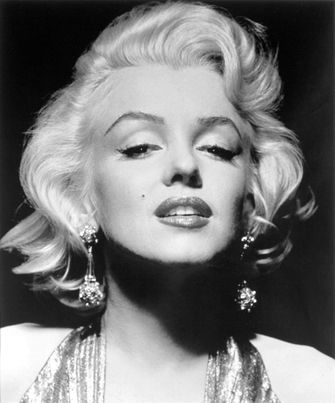
These are the images that I tried.
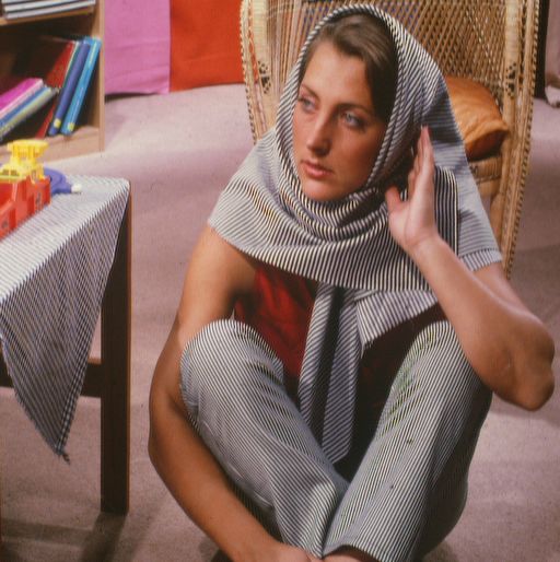  
Barbara: found both color and bw copies and a slightly cropped version.
Marilyn: found cropped and stretched versions, and an even edited (defaced) version.
Lenna: found both color and bw, but not partial or rotated versions (even though a rotated version is in the index).
May 12, 2008
Let’s review part 1 first. If you have a 100×100 gray scale image, it is simply a table of 100×100 = 10,000 numbers. You rearrange the rows of this table into a 10,000-vector and represent the image as a point in the 10,000-dimensional Euclidean space. This enables you to measure distances between images, discover patterns, match images, etc. Now, what is wrong with this approach?
Suppose A, B, and C are images with a single black pixel in the left upper corner, next to it, and the right bottom corner respectively. Then, the distances will be the equal: d(A,B) = d(B,C) = d(C,A), no matter how you define the distance d(,) between points in this space. The conclusion: if A and B are in the same cluster, then so is C. So adjacency of pixels and distance between them is lost in this representation!
Of course this can be explained, as follows. The three images are essentially blank so it’s not surprising that they are close to the blank image and to each other. So as long as pixels are “small” the difference between these four images is justifiably negligible.
Of course, “small” pixels means “small” with respect to the size of the image. This means high resolution. High resolution means larger image (for the same “physical” object), which means higher dimension of the Euclidean space, which means higher computational costs. Not a good sign.
To take this line of thought all the way to the end, we have to ask the question: what if we keep increasing resolution?
The image will simply turn into an exact copy of the “physical” object. Initially, the image is a table of numbers. Now, you can think of the table as a rectangle subdivided into small squares, then the image is a function to the reals constant on each of these squares. As the resolution grows, the rectangle remains the same but the squares become smaller. In the end we have a - possibly continuous – function (as the limit of this sequence of functions). This is the “real” image and the rest are its approximations.
It’s not as clear what happens to the representations of images in the Euclidean space. The dimension of this space grows and in the end becomes infinite! It also seems that this new space should be made of infinite strings of numbers. That does not work out.
Indeed, consider this (“real”) image: a white square with a black upper left quarter. Let’s represent it first as a 2×2 image. Then in the 4-dimensional Euclidean space this image is (1,0,0,0). Now let’s increase the resolution. If this is a 4×4 image, it is (1,1,0,0,1,1,0,0,..,0) in the 16-dimensional space. In the 32-dimensional space it’s (1,1,1,1,0,0,0,0,1,1,1,1,0,0,0,0,1,1,1,1,0,…,0). You can see the pattern. But what is the end result (as the limit of this sequence of points)? It can’t be (1,1,1,…), can it? It definitely isn’t the original image. That image can’t even be represented as a string of numbers, not in any obvious way…
OK, these are just signs that there may be something wrong with this approach. A more tangible problem is that unless the two images are aligned first, there is no way to use this representation to discover that they depict the same or similar thing. About that in the next post.
May 2, 2008
I read this press release a few weeks ago. Just like many others it presents some over-optimistic report of a new method that is supposed to solve a problem. Just like many others it’s about face recognition. For a change I decided to read the paper the report is based on and write up my thoughts.
First, the paper itself is much more modest that the press release. That’s very common. Let’s look closer.
The traditional approach to face identification is to look for distinctive features – eyes, nose, mouth - and then match them with those of the other image or images. Here approach is to take everything in the image, every “feature”. First, let’s make this clear: when they say “features” they mean simply pixels! I have no idea why… They also don’t emphasize the obvious consequence – the method should work with any images not just faces.
This language of “features” obscures a common and straightforward approach to data representation and pattern recognition, as follows. Suppose you have a collection of 100×100 images. Then you rearrange the rows of this 100×100 “matrix” into a 10,000-vector. As a result, each image is represented as a point in the 10,000-dimensional space. This is clearly a brute force approach. However, something like that is inevitable if you don’t have an insight into the nature of the problem. Once all the data is in a Euclidean space (no matter how large), all statistical, data processing and pattern recognition methods can be used. Nice! The most common method is probably clustering – looking for groups of points unusually close to each other.
I have always felt OK about this approach but this time I started to doubt its applicability in analysis of images.
First you notice is that this approach can only work as long as all images have the same dimensions. It gets trickier if you study images of different dimensions. For example, if you had both 30×20 images and 1×600 images in the collection, that would really mess up everything! In a less extreme case, the presence of 30×20 and 20×30 images in the collection would be a problem. Of course you can simply add extra blank pixels up to 30×30 as a “common denominator”. However, it appeared to me that such a problem (and such an awkward solution) may be an indication of bigger issues with the whole approach.
I asked myself, does this approach preserve the structural information contained in the image? The very first thing to look at is the adjacency of pixels. Since each pixel corresponds to an independent dimension, it seems that the adjacency is still contained in those coordinates: (a,b,…) is not the same as (b,a,…). Wrong!
It suffices to look at the distance between points – images - in this 10,000-dimensional space. It can be defined in a number of ways, but as long as it is symmetric we have a problem. Suppose the distance between (1,0,…,0) and (0,1,0,…,0) is d. Then the distance between (1,0,…,0) and (0,0,…,0,1) is also d. Here (1,0,…,0) and (0,1,0,…,0) are two images with a single pixel in each – located adjacent to each other - while (0,0,…,0,1) has a pixel in the opposite corner! The result is odd and you have to ask yourself, can clustering be meaningful here?
More to come…
— Next Page » |
|
|


")


