TinEye is an image-to-image search engine from Idée. It is in a closed testing but I got to try it a couple of days ago. After a very positive review at TechCrunch, I decided to write up my impressions (a review of an earlier version is here).

They don’t make wild claims about being able to do face identification or similar (unsolved) problems. The goal seems very simple: find copies of images. With this task TinEye does a fairly good job. It finds even ones that have been modified - noise, color, stretch, crop, some photoshopping. It does not do well with rotation. That’s a major drawback (compare to Lincoln from MS Research).

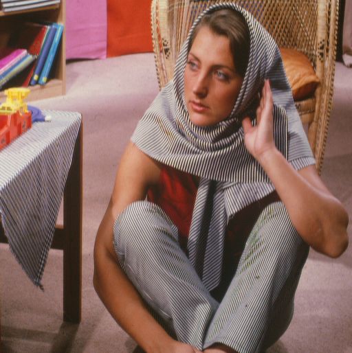
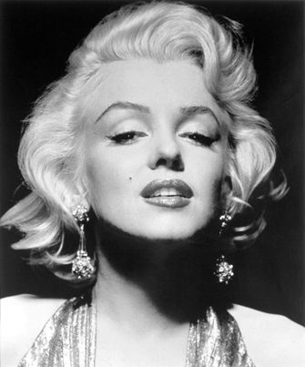
These are the images that I tried.

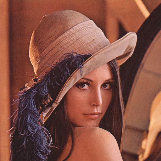
Barbara: found both color and bw copies and a slightly cropped version.

Marilyn: found cropped and stretched versions, and an even edited (defaced) version.

Lenna: found both color and bw, but not partial or rotated versions (even though a rotated version is in the index).

We are happy to announce the release of cellAnalyst version 2.0!

Just to remind you, cellAnalyst by AssaySoft Inc. is an advanced image-mining tool in a user-friendly package. It is designed to automate the analysis of digital images, especially ones coming from cell biology. It works as follows:

1. The images are initially presented in a photo album format.
2. With just a few clicks, cells have been detected, captured, and measured.
3. The cells are listed in a table along with their characteristics.
4. Each such table is saved as an entry in a searchable database.

Items 2 and 3 came originally from Pixcavator.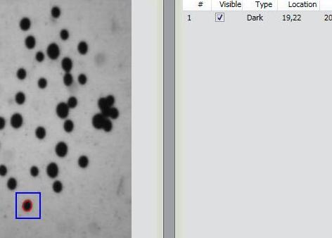

Now, the main new feature in version 2.0 is Partial Analysis. Analysis of images may be a time consuming task especially when the analysis setting have to be determined by trial and error. To reduce the processing time, one may start with analysis of just a portion of the image. The user draws a rectangle around a cell, and the analysis instantly determines its size and contrast. These two numbers are then used as the settings for the analysis of the entire image. More will appear in the wiki under Analysis strategy.

Other improvements are these:

• The roundness of every object found in the image is computed and displayed in the output table.
• Image enhancement functions are added: you can adjust brightness, contrast, color balance, gamma correction, and saturation.
• The estimated processing time is computed and displayed so that the user can plan ahead.
• Annotation can be added to images; it can later be used for search.

Download cellAnalyst here.

Feedback will be appreciated!

Let’s review part 1 first. If you have a 100×100 gray scale image, it is simply a table of 100×100 = 10,000 numbers. You rearrange the rows of this table into a 10,000-vector and represent the image as a point in the 10,000-dimensional Euclidean space. This enables you to measure distances between images, discover patterns, match images, etc. Now, what is wrong with this approach?

Suppose A, B, and C are images with a single black pixel in the left upper corner, next to it, and the right bottom corner respectively. Then, the distances will be the equal: d(A,B) = d(B,C) = d(C,A), no matter how you define the distance d(,) between points in this space. The conclusion: if A and B are in the same cluster, then so is C. So adjacency of pixels and distance between them is lost in this representation!

Of course this can be explained, as follows. The three images are essentially blank so it’s not surprising that they are close to the blank image and to each other. So as long as pixels are “small” the difference between these four images is justifiably negligible.

Of course, “small” pixels means “small” with respect to the size of the image. This means high resolution. High resolution means larger image (for the same “physical” object), which means higher dimension of the Euclidean space, which means higher computational costs. Not a good sign.

To take this line of thought all the way to the end, we have to ask the question: what if we keep increasing resolution?

The image will simply turn into an exact copy of the “physical” object. Initially, the image is a table of numbers. Now, you can think of the table as a rectangle subdivided into small squares, then the image is a function to the reals constant on each of these squares. As the resolution grows, the rectangle remains the same but the squares become smaller. In the end we have a - possibly continuous – function (as the limit of this sequence of functions). This is the “real” image and the rest are its approximations.

It’s not as clear what happens to the representations of images in the Euclidean space. The dimension of this space grows and in the end becomes infinite! It also seems that this new space should be made of infinite strings of numbers. That does not work out.

Indeed, consider this (“real”) image: a white square with a black upper left quarter. Let’s represent it first as a 2×2 image. Then in the 4-dimensional Euclidean space this image is (1,0,0,0). Now let’s increase the resolution. If this is a 4×4 image, it is (1,1,0,0,1,1,0,0,..,0) in the 16-dimensional space. In the 32-dimensional space it’s (1,1,1,1,0,0,0,0,1,1,1,1,0,0,0,0,1,1,1,1,0,…,0). You can see the pattern. But what is the end result (as the limit of this sequence of points)? It can’t be (1,1,1,…), can it? It definitely isn’t the original image. That image can’t even be represented as a string of numbers, not in any obvious way…

OK, these are just signs that there may be something wrong with this approach. A more tangible problem is that unless the two images are aligned first, there is no way to use this representation to discover that they depict the same or similar thing. About that in the next post.

After Google “launched” its ImageRank - by presenting a paper about it, now there are two more.

First, Idée “publicly launched” its image search engine (report here). If you want to try it, they’ll put you on a waiting list. How is it different from what we saw before?

Second, “Pixsta launches image search engine” (report here). Testing is also closed. What is the difference from what we saw before?

The only good thing here is that I discovered a better term for visual image search, CBIR, etc. It’s “image-to-image search“, as opposed to text-to-text and text-to-image we are familiar with.

I’ve tried a variety of images and, as the diagram indicates, the processing time appears to depend linearly on the number N of pixels in the image. Roughly, 40 seconds for each million pixels in the image. The testing was done on HP Pavilion laptop with Intel Core 2 Dual CPU T7500 2.2GHz.

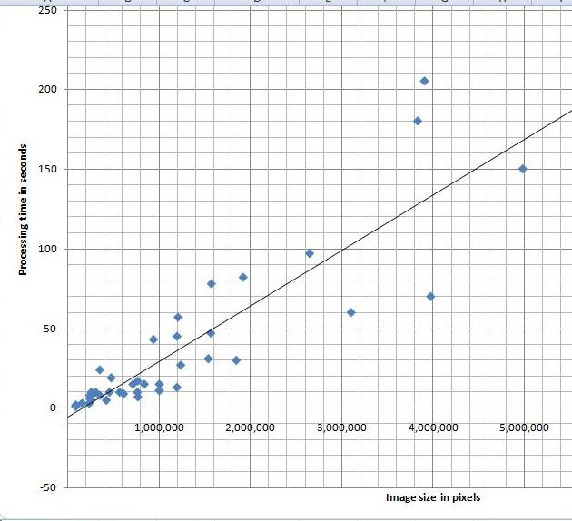
I can’t improve my estimate though. It’s O(N^2) (link to the article in Wikipedia). That’s how we get it. The analysis algorithm works as follows: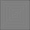

• Each pixel is processed separately.
• For each of the N pixels an object is created and you may have to run around it to mark its edges.
• If this object is very thin and fills the image (like this spiral), its perimeter is proportional to N.

My feeling is that the images of this kind are unusual. Maps may be close, as well as microchips, or anything fractal-like. Cells are OK.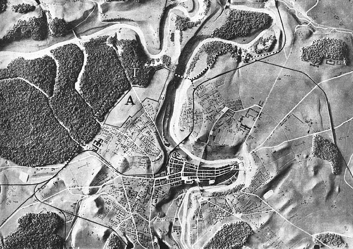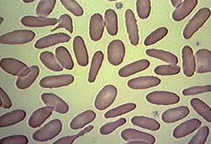

Update: The estimate O(N^2) refers to the time of image analysis - creation of the graph. After that, you still have to run up and down this graph to come up with the output data. BTW, the size of the graph and, therefore, the memory depends linearly on N, O(N).

I read this press release a few weeks ago. Just like many others it presents some over-optimistic report of a new method that is supposed to solve a problem. Just like many others it’s about face recognition. For a change I decided to read the paper the report is based on and write up my thoughts. 

First, the paper itself is much more modest that the press release. That’s very common. Let’s look closer.

The traditional approach to face identification is to look for distinctive features – eyes, nose, mouth - and then match them with those of the other image or images. Here approach is to take everything in the image, every “feature”. First, let’s make this clear: when they say “features” they mean simply pixels! I have no idea why… They also don’t emphasize the obvious consequence – the method should work with any images not just faces.

This language of “features” obscures a common and straightforward approach to data representation and pattern recognition, as follows. Suppose you have a collection of 100×100 images. Then you rearrange the rows of this 100×100 “matrix” into a 10,000-vector. As a result, each image is represented as a point in the 10,000-dimensional space. This is clearly a brute force approach. However, something like that is inevitable if you don’t have an insight into the nature of the problem. Once all the data is in a Euclidean space (no matter how large), all statistical, data processing and pattern recognition methods can be used. Nice! The most common method is probably clustering – looking for groups of points unusually close to each other.

I have always felt OK about this approach but this time I started to doubt its applicability in analysis of images.

First you notice is that this approach can only work as long as all images have the same dimensions. It gets trickier if you study images of different dimensions. For example, if you had both 30×20 images and 1×600 images in the collection, that would really mess up everything! In a less extreme case, the presence of 30×20 and 20×30 images in the collection would be a problem. Of course you can simply add extra blank pixels up to 30×30 as a “common denominator”. However, it appeared to me that such a problem (and such an awkward solution) may be an indication of bigger issues with the whole approach.

I asked myself, does this approach preserve the structural information contained in the image? The very first thing to look at is the adjacency of pixels. Since each pixel corresponds to an independent dimension, it seems that the adjacency is still contained in those coordinates: (a,b,…) is not the same as (b,a,…). Wrong!

It suffices to look at the distance between points – images - in this 10,000-dimensional space. It can be defined in a number of ways, but as long as it is symmetric we have a problem. Suppose the distance between (1,0,…,0) and (0,1,0,…,0) is d. Then the distance between (1,0,…,0) and (0,0,…,0,1) is also d. Here (1,0,…,0) and (0,1,0,…,0) are two images with a single pixel in each – located adjacent to each other - while (0,0,…,0,1) has a pixel in the opposite corner! The result is odd and you have to ask yourself, can clustering be meaningful here?

More to come…