This site contains: mathematics courses and book; covers: image analysis, data analysis, and discrete modelling; provides: image analysis software. Created and run by Peter Saveliev.

From Intelligent Perception

Cell complexes appear in real life, see Cells and cell complexes.

We have used cubical complexes as topological spaces made of simple pieces and, therefore, an appropriate subject for quantitative analysis, specifically, homology. These pieces are, in 2d, squares and segments on the grid.

Now, the best simplest complex we could use to represent a topological circle is four edges arranged in a square. But why should we need four pieces when we know that a circle is built from a single segment with the end-points glued together?

This last construction is very simple. Initially the (cubical) complex $K$ is:

• $0$-cells: $A, B$,
• $1$-cells: $a$,
• boundary operator: $\partial a = A + B$.

Then we identify $A$ and $B \colon A \sim B$. The new complex $S$ is:

• $0$-cells: $A$;
• $1$-cells: $a$;
• boundary operator: $\partial a = 0$.

Certainly, this is not a cubical complex because we can't place these cells on the grid. However, the possibility of algebraic analysis remains since boundary operator can still be computed: $$\partial a = A + A = 0.$$

Further, the chain complex of $S$ is generated by $a$ and $A$:

• $C_0(S) = <A>$,
• $C_1(S) = <a>$,
• boundary operator: $\partial = 0 \colon C_1(S) \rightarrow C_0(S)$.

Then the homology $H_*(S)$ of $S$ is generated by the homology classes of $a$ and $A \colon [a], [A]$. Hence:

• $H_0(S) = {\bf Z}_2,$
• $H_1(S) = {\bf Z}_2.$

Observe now that the cells in a cubical complex are "open", i.e., homeomorphic to open balls, while the cells in a cell complex are "closed", i.e., homeomorphic to closed balls. The reason is that a cubical complex is built as a union of disjoint cells while the cells in a cell complex are glued to each other along their boundaries. A cubical complex can be interpreted as a cell complex in the obvious way.

Example. Let's consider how we build the cylinder from the square.

The complex $K$ of the square is:

• $0$-cells: $A, B, C, D$;
• $1$-cells: $a, b, c, d$;
• $2$-cells: $\tau$;
• boundary operator: $\partial \tau = a + b + c + d; \partial a = A + B, \partial b = B + C$, etc.

Recall, we create the cylinder $C$ by gluing two opposite edges with the following equivalence relation: $$(0,y) \sim (1,y).$$

Now, what about complexes? Can we interpret the gluing as equivalence of $a$ and $c$? Yes, but we also have to take care of the other cells as well:

• $a \sim c;$
• $A \sim D, B \sim C.$

Once again, this is not a cubical complex! However, the we still have our collection of cells (with some identified), only the boundary operator is different:

• $\partial \tau = a + b + c + d = a + b + a + d = b + d;$
• $\partial a = A + B, \partial b = B + C = 0, \partial c = A + B, \partial d = D + A = 0.$

Now, the chain complex of $K$ can be defined and its homology computed. The second line indicates that $b$ and $d$ are cycles and the first indicates that they are homologous. Hence $$H_1(C)= {\bf Z}_2.$$

Example. Suppose now that we want to build the Mobius band ${\bf M}^2$. The equivalence relation is given by $$(0,y) \sim (1,1-y).$$

Once again we can interpret the gluing as equivalence of $a$ and $c$. But this time they are attached to each other with $c$ upside down. It makes sense then to interpret this as an equivalence of cells but with a "twist": $$a \sim -c.$$ Here $-c$ represents edge $c$ with the opposite orientation. Further $$A \sim D, B \sim C.$$

The boundary operator is:

• $\partial \tau = a + b + c + d = a + b - a + d = b + d;$
• $\partial a = A + B, \partial b = B + C = 0, \partial c = A + B, \partial d = D + A = 0.$

Same as for the cylinder! Hence $$H_1({\bf M}) = {\bf Z}_2.$$

So, a cell complex is something built from cells via a quotient. This approach allows us to ignore the question of whether or not it fits into a Euclidean space.

How do we attach the cells to each other? Remember we want to be able to compute the boundary operator. Since the boundary of a $k$-cell is made of $(k-1)$-cells, we will only allow to attach $k$-cells to $(k-1)$-cells.

For example, suppose we already have a complex with two $0$-cells $A, B$ and a $1$-cell $a$. How can we add a new $1$-cell $b$ to $K$? First, we can't attach an end point of $b$ to the middle of $a$. This point can only be a $0$-cell that is already present in the complex.

Then, there are $4$ proper ways we can do that:

• from $A$ to $B$,
• from $A$ to $A$,
• from $B$ to $B$.

If we have a collection of cells of various dimensions, the general procedure of building a cell complex is:

1. start with $0$-cells,
2. attach the end points of $1$-cells to the $0$-cells,
3. attach the $2$-cells to the $1$-cells,
4. etc.

At the end of $n$-th step you have the $n$-th skeleton $K_n$ of $K$.

Example. Suppose these are the cells:

• $0$-cells: $A, B, C, D$;
• $1$-cells: $a, b, c$;
• $2$-cells: $\tau$.

One way to build a cell complex from these parts is this:

Now we can compute the boundary operator based on this procedure:

• $\partial \tau = a + b;$
• $\partial a = A + B, \partial b = A + B, \partial c = 0.$

Note: We can almost recover the whole complex from the boundary operator! The only ambiguity is that $c$ can be attached (this way) to any $0$-cell, not just $D$.

The formal definition of a cell complex is inductive.

Definition. Suppose we have a finite collection of (abstract) cells $K$. Suppose $C_n$ denotes all $n$-cells in $K$. Next, the $0$-skeleton $K_0$ is defined as the disjoint union of $0$-cells: $$K_0 = \bigcup C_0.$$ Suppose that the $n$-skeleton $K_n$ has been constructed. Then the $(n+1)$-skeleton $K_{n+1}$ is constructed as follows. Suppose for each $(n+1)$-cell a there is a gluing map $$f_a \colon \partial a \rightarrow K_n.$$ Then all $(n+1)$-cells are "added" to $K_n$ resulting in the $(n+1)$-skeleton $K_{n+1}$ defined as the disjoint union of the $n$-skeleton $K_n$ and all the $(n+1)$-cells, under a certain equivalence relation: $$K_{n+1} = (K_n \bigcup C_{n+1})/ _{\sim},$$ where $\sim$ is defined by:

The gluing maps have to satisfy an extra condition: $$f_a(\partial a) {\rm \hspace{3pt} is \hspace{3pt} the \hspace{3pt} union \hspace{3pt} of \hspace{3pt} a \hspace{3pt} collection \hspace{3pt} of \hspace{3pt} cells \hspace{3pt} of \hspace{3pt}} K.$$

Thus, cell complex $K$ is a combination of the cells, the skeleta, and the gluing maps.

Note that without the extra condition the result is called a CW complex. As you can see in the illustration, the results may differ (not homeomorphic). However, the spaces are "homotopy equivalent" and, therefore, the homology (as well as all other algebraic topological invariants) coincide. The point of this condition is to allow us to proceed directly to algebra. For example, if the (topological) boundary of an $(n+1)$-cell $\tau$ is identified with the union of $n$-cells $a, b, c$, then the (algebraic) boundary of $\tau$ is the sum of $a, b, c$: $$f_{\tau}(\partial \tau) = a \cup b \cup c \rightarrow \partial \tau = a + b + c.$$

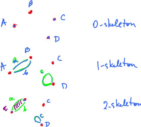
Example. The image below illustrates the three steps of the construction of a cell complex with cells of dimension $0$ and $1$.

Example. Consider examples of building a $2$-skeleton from the same $1$-skeleton (on the right). Suppose these are the cells:

• $0$-cells: $A, B, C, D$;
• $1$-cells: $a, b, c$;
• $2$-cells: $\tau$.

We can define the gluing map for dimension $1$ based an the boundary operator:

• $\partial a = A + B$,
• $\partial b = B + C,$
• $ \partial c = C + A.$

Indeed, suppose $a=[0,1]$. Then $f_a(0) = A$ and $f_a(1) = B$. Then $0 \sim A$ and $1 \sim B$. Similar for $b$ and $c$. The result is $K_1$.

Now suppose we are to attach $\tau$ to $K_1$.

Now we need to choose the gluing map for dimension $2$: $$f_{\tau} \colon \partial \tau \rightarrow K_1 {\rm \hspace{3pt} or \hspace{3pt}} f_{\tau} \colon {\bf S}^1 \rightarrow {\bf S}^1.$$

The choice of this map may be vary. The obvious choice is a homeomorphism.

Then $\tau$ is like a film of the frame made of $a, b,$ and $c$. The end result, the $2$-skeleton $K_2$, is homeomorphic to the disk.

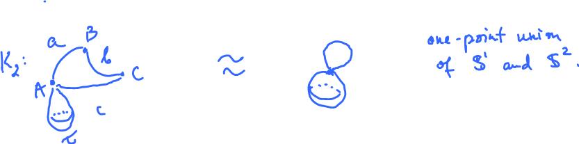
What if the gluing map $f_{\tau} \colon {\bf S}^1 \rightarrow {\bf S}^1$ isn't a homeomorphism? The simplest choice is a constant map, for example: $$f_{\tau}(x) = A {\rm \hspace{3pt} for \hspace{3pt} all \hspace{3pt}} x \in \partial a.$$

Then $$x \sim A {\rm \hspace{3pt} for \hspace{3pt} all \hspace{3pt}} x \in \partial a,$$

i.e., the whole $\partial a$ is glued to $A$. Such gluing produces a sphere ${\bf S}^2$.

Exercise. Find other other possibilities for the gluing map $f_{\tau}(x)$ and sketch the resulting complexes.

For more examples, read Examples of cell complexes.

Theorem. $A$ finite (i.e., one with finitely many cells) is compact.

Proof. It is easy to see that a finite (disjoint) union of compact spaces is compact. So the initial union $X$ of the cells of the complex is compact. Now $K = X/ _{\sim}$, thence $K$ is compact as a quotient of a compact space (indeed, it's the image of a compact space under a continuous map). $\blacksquare$