This page is a part of CVprimer.com, a wiki devoted to computer vision. It focuses on low level computer vision, digital image analysis, and applications. It is designed as an online textbook but the exposition is informal. It geared towards software developers, especially beginners, and CS students. The wiki contains mathematics, algorithms, code examples, source code, compiled software, ans some discussion. If you have any questions or suggestions, please contact me directly.
Tutorial
From Computer Vision Primer
Tutorial on how to use Pixcavator (the official download page is here). Compare to other Image analysis software.
Contents |
Overview

Pixcavator [1] is an image analysis program for scientists and researchers. It captures objects in the image by means of contours (outlines) and produces an Excel spreadsheet with those objects locations and measurements.
The processing goes through three main stages:
- Stage 1: automatic. A graph is created that contains complete data about the image.
- Stage 2: semi-automatic. The user moves sliders corresponding to objects’ characteristics to instantly change their boundaries and choose the best segmentation. The output data is updated in real time.
- Stage 3: manual. The user can exclude noise and irrelevant details from the analysis by simply clicking on them.
Currently, Pixcavator has the following tabs.
- Analysis allows the user to load the image and start the analyze.
- Tools allows the user to manipulate the image using common image processing tools and special effects
- Output allows the user to view, explore and save the output data and the updated image.
Load an image and set up analysis
Start at the Analysis tab.
Select an image file from your computer by using the Choose image… button on the right. Most popular formats are supported: JPEG, BMP, PNG, GIF, TIFF.
The image will appear in the window on the left.
You can pan it using the left button of your mouse. The right button provides you with a magnification tool.
Note: when you open a new image, the previous analysis data is discarded.
Analysis of large images will take longer. The estimated processing time (2.4 GHz, Pentium 4) for gray scale images may be estimated by:
40 * width of the image * height of the image / 1000,000 seconds.
This data is displayed on the right. Simpler images take less time, complex more. It will take about 25 seconds to process a gray scale 512×512 image. See Processing time.
If you are interested mainly in image analysis, smaller details within the image may be of relatively low interest. If this is the case, consider shrinking the image.
Use the slider marked with Shrink factor.
It is important to understand that both dimensions of the image are reduced. Therefore, if the slider is set at m, each of the two the dimensions of the image will be shrunk by m. Therefor the size will be reduced by m*m. For example, if you set the slider at 2, the processing time will be cut by a factor of 2*2=4.
For your convenience, this slider is preset so that the processing time is under 10 seconds. The use of this option is also appropriate for the initial analysis of a large image before you commit yourself to a long wait.
Keep in mind that once the image is shrunk, it is the new image that will be analyzed. Generally, this will not affect the number of objects detected as long as they are "large" and stay apart from each other. However, the sizes and locations of the objects will be displayed relative to the shrink coefficient.
Example. If an object has size 100 (100 pixels) in the original image and the shrink coefficient is 2, then the size displayed will be 25.
Example. If an object is located at X=100, Y=100 in the original image and the shrink coefficient is 2, then the location displayed will be (50,50).
Another way of thinking about shrinking the image is as reducing image resolution.
For more on this and examples of how to deal with shrinking and scaling, see Calibration.
There is another way to improve the processing speed. Using the image processing tools (below) crop a small but important portion of the image and analyze it. This will remove the unwanted clutter in the image and will make the analysis more meaningful.
Choose also the RGB channel you want to be analyzed.
Modify the image with image processing tools
Even if your interest is only in image analysis, you may want to try to modify the image with some image processing tools.
Go to the Tools tab. The image on the left is the original and the one on right will show the effects of these operations. You can enhance the original image before analyzing it or enhance the simplified image after analyzing it.
You can adjust the image’s Brightness, Contrast, Hue, and Saturation by using the sliders on the left. This may enhance the image.
On the right, there is a drop down menu for Filters and effects.
- The most important tools for image analysis are at the top – Basic tools: Dilation and erosion, Crop, Subtract, Add border, Blur, Median filter, Noise, etc.
Some of these add imperfections to the image. They simulate real life effects and can be used to test the robustness of image analysis.
The rest of the items in this menu add artistic effects to the image.
For more see Pixcavator's image processing tools.
Analyze the image and view output
Process the image by pressing Run in the Analysis tab.
You can pan with the left button of your mouse and magnify with the right button.
In the Output tab the updated image is now displayed on the left. Each object that has been detected is captured with a contour. Dark objects are outlined with red and light with green. To understand how they are found, read Boundaries in gray scale images.
If you click within the image while holding Ctrl, the nearest object to your mouse will be marked or unmarked. If, in addition, you move the mouse, the objects close to the rectangle spanned this way will be marked or unmarked. As a result, the corresponding squares or contours will appear or disappear.
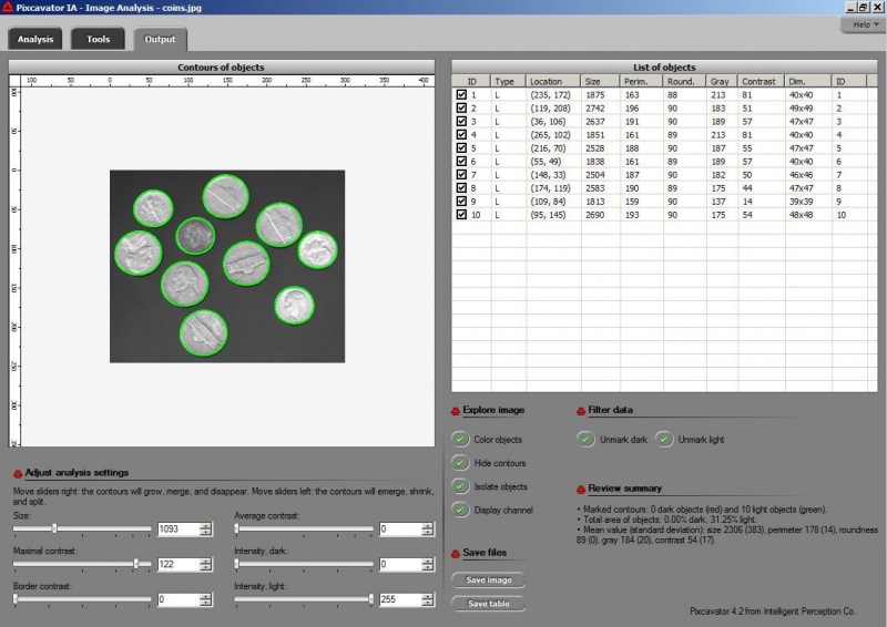
On the right, there is a table containing all objects in the image satisfying the analysis restrictions. For each objects the following data is displayed:
- light or dark,
- location (coordinates of the centroid = the center of mass of the object as a lamina of uniform density),
- size (the number of pixels = area),
- perimeter,
- roundness (above 80 for circles, less for everything else),
- intensity (max/min level of gray),
- location of the center of mass (of the object as a lamina with density = gray level), -- not currently
- average contrast (saliency/size),
- thickness and length.
For more on nature of these parameters and for examples on how to use these parameters see Measuring objects, Areas of objects, Centroid, Contrast, Roundness, Saliency, Center of mass, Thickness and length, etc. See also Computation error.
Changing analysis settings with sliders

There are three sliders on the left that allow you to edit the analysis settings. The objects that fall below these thresholds will be ignored by the analysis procedure and not counted. To understand what we consider an object in an image read Objects in gray scale images.
First, choose a threshold for Size. For example, if you choose 100, every object containing less than 100 pixels will not captured or counted. The Size slider is set automatically depending on the size of the image.
Second, choose a threshold for Contrast. For example, if you choose 20, every object surrounded by an area with gray level that differs from that of the object by less than 20 will be ignored. There are 256 levels of gray.
Third, use the Max growth rate slider. Recall the object in the image are allowed to grow – from one level of gray to the next - up to the extent set by the slider (see Boundaries in gray scale images). For example, the object will grow until it’s both larger than say 100 pixels and has contrast above 20. This slider is very different from the other two. If you choose 10, the object will be allowed to expand – from one level of gray to the next - as long as its size grows by 10% or less. Roughly, the expansion stops once the contour reaches a sharp edge. (To reproduce results you obtained with versions 3.0 and earlier, keep this value at 0.)
If the analysis results are unsatisfactory, you don't have to start over!
You can experiment with the settings and the table and contours are updated almost instantly every time you move the sliders.
Explore output image and data
Just like with any spreadsheet, if you click a column header, the rows in the table will be sorted from high to low or low to high with respect to the entries in this column.
To mark and unmark a row in the table, check and uncheck the square in the beginning of the row. If an object is marked or unmarked in the table on the right, a contour appears or disappears around it in the image on the left, and vice versa.
You can erase everything outside the marked objects by pressing Isolate objects. See Background removal.

You can randomly color objects, marked only. See Coloring objects.
You can hide contours. To see the original image you used to have to go to the Analysis tab. Now you can flick it on and off to see what is hiding under the contours. The marking/unmarking of objects is unaffected.
In Pixcavator PE you can Simplify the image by filling the contours (or squares) of unmarked objects with the corresponding level of gray. That level is chosen equal to the intensity of the border of the object. See Image Simplification.
Analysis summary. The output table contains only the raw data about each object. Of course, if you save the data to Excel, you can get anything from it: average of all columns, histograms, etc. We thought that it would be nice to be able to preview some data: average values of size and contrast. The analysis summary includes the Mean values and Standard deviations of all the main characteristics of objects (marked only).
Hover over an object and view its data. It's displayed right under the image. That’s a new, convenient feature. You used to have to mark/unmark object in the image and then find the row in the table to see the object's measurements. That’s not a good idea if the table is a hundred rows long. Now you let the mouse hover over the object of your interest and the data from the table is displayed right beneath the image.
A new header is Data filtering. There are only two buttons here currently – Unmark dark and Unmark light. For convenience they were redesigned as follows. These are toggle buttons so that you can choose to concentrate on only, say, light objects. You don't have to unmark dark every time you change the settings. There is more to come here.
You can save the displayed image - with all contours or squares, all marked, unmarked, or isolated objects – by pressing Save image. Finally, you can export the output table to Excel by pressing Save table.
Notes
Also, read Analysis strategy and Filtering output data.
Another exposition of this material is in the User Guide.
For examples take a look at our image gallery. See also Human vision vs. computer vision.
Read about real-life applications of Pixcavator under Case studies and Projects.
Top finds
- Casinos Not On Gamstop
- Non Gamstop Casinos
- Casino Not On Gamstop
- Casino Not On Gamstop
- Non Gamstop Casinos UK
- Casino Sites Not On Gamstop
- Siti Non Aams
- Casino Online Non Aams
- Non Gamstop Casinos UK
- UK Casino Not On Gamstop
- Non Gamstop Casino UK
- UK Casinos Not On Gamstop
- UK Casino Not On Gamstop
- Non Gamstop Casino UK
- Non Gamstop Casinos
- Non Gamstop Casino Sites UK
- Best Non Gamstop Casinos
- Casino Sites Not On Gamstop
- Casino En Ligne Fiable
- UK Online Casinos Not On Gamstop
- Online Betting Sites UK
- Meilleur Site Casino En Ligne
- Migliori Casino Non Aams
- Best Non Gamstop Casino
- Crypto Casinos
- Casino En Ligne Belgique Liste
- Meilleur Site Casino En Ligne Belgique
- Bookmaker Non Aams
- カジノ ライブ
- онлайн казино с хорошей отдачей
- スマホ カジノ 稼ぐ
- ブック メーカー オッズ
- Top 3 Nhà Cái Uy Tín Nhất
- Trang Web Cá độ Bóng đá Của Việt Nam
- Casino En Ligne Avis
- Casino En Ligne France
- Casino En Ligne
- 꽁머니 토토
- Casino Online Non Aams
- Meilleur Casino En Ligne
